Hydraulic Fracturing Fundamentals

58 minutes read

Fracturing fluids types, Fracture geometry, Frac job design, Hydraulic fracturing techniques, Fracture propagation, Fracking equipment, Fracturing fluid composition, Hydraulic fracturing explained, Fracking techniques, Hydraulic fracturing process, Hydraulic Fracturing, Fracking, Shale Gas Extraction, Fracture Stimulation, Fracturing Fluids, Proppants, Unconventional Oil and Gas, Hydraulic Fracturing Process, Frac Jobs, Fracture Network, Fracture Propagation, Horizontal Drilling, Hydraulic Fracturing Wells, Frac Sand, Well Stimulation, Shale Formation, Fracture Fluids, Fracture Treatment, Fracture Pressure, Reservoir Stimulation, Fracture Design, Fracture Width, Fracture Monitoring, Fracture Optimization, Fracture Mechanics, Hydraulic Fracturing Fundamentals

Quantitative Description of Fracture Growth

Fracture models are attempts to describe the dimensions of hydraulically created fractures based on particular combinations of fluid volumes, fluid properties, injection rates, injection pressures and formation mechanical properties. If a model can define fracture dimensions relatively accurately for these combinations of parameters, then the rates and pressures required to attain desired fracture geometries can be determined, and a fracturing treatment designed accordingly. When combined with estimates of the expected improvement in productivity resulting from a fracture of specific geometry, it is possible to economically optimize well performance and hydraulic fracturing investments.

Two-Dimensional Mathematical Models

Three factors compete for the fluid volume remaining in a fracture after leakoff:

Lateral extent of the fracture wing
Fracture height
Fracture width

Simple 2-D mathematical models assume that either the fracture height is a constant value or that the fracture extends vertically and horizontally with the same radial dimension. Once the problem is reduced to two dimensions, additional assumptions are applied to determine a relationship between fracture extent and fracture width.

The final equations for each of these models are derived from the concept that the viscous resistance to flow gives rise to a net pressure that is exerted on the fracture faces and keeps the fracture open. It is not surprising, therefore, that fracture width is related to such variables as elastic modulus, injection rate, viscosity of the fracturing fluid and fracture length.

Two-dimensional models commonly used for describing hydraulic fractures include:

The Perkins – Kern – Nordgren (PKN) model
The Kristianovich – Zheltov – Geertsma – DeKlerk (KGD) model
The radial model

Perkins-Kern-Nordgren (PKN) Model

Perkins and Kern developed a 2-D model for hydraulic fractures which was modified by Norgden and has become known as the “PKN” model. The visual representation underlying the PKN model is a two-wing rectangular fracture of constant height with a vertical cross section that is an ellipse (Figure 1).

Perkins-Kern-Nordgren model, Hydraulic Fracturing, Fracturing fluids types, Fracture geometry, Frac job design, Hydraulic fracturing techniques, Fracture propagation, Fracking equipment, Fracturing fluid composition, Hydraulic fracturing explained, Fracking techniques, Hydraulic fracturing process, Hydraulic Fracturing, Fracking, Shale Gas Extraction, Fracture Stimulation, Fracturing Fluids, Proppants, Unconventional Oil and Gas, Hydraulic Fracturing Process, Frac Jobs, Fracture Network, Fracture Propagation, Horizontal Drilling, Hydraulic Fracturing Wells, Frac Sand, Well Stimulation, Shale Formation, Fracture Fluids, Fracture Treatment, Fracture Pressure, Reservoir Stimulation, Fracture Design, Fracture Width, Fracture Monitoring, Fracture Optimization, Fracture Mechanics — **Figure 1**: Perkins-Kern-Nordgren model

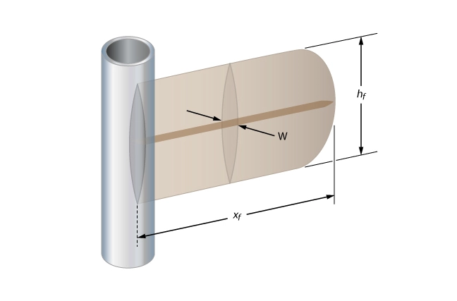
The maximum width of the ellipse at a certain distance from the well is related to the height, plane strain modulus and net pressure at that location. Since the net pressure is also related to injection rate and fluid viscosity, a width equation not containing the pressure can be derived. Of particular interest is the maximum width of the ellipse located at the wellbore, defined by

$W _{w,0} = 3.27\, \left( \dfrac{\mu \, q_i\, x_f}{E'} \right)^\frac{1}{4}$

Where

$W_{w,0} =$ maximum fracture width at center point of wellbore

$E' =$ Young’s modulus (modulus of elasticity of rock)

$q_i =$ injection rate

$\mu =$ viscosity of injected fluid

$x_f =$ fracture half-length

The constant was 3.57 in the original Perkins-Kern form of the equation, but the above form given by Nordgren is more generally accepted. The average width of the fracture $(\overline{w})$ is related to the maximum as follows:

Kristianovich – Zheltov – Geertsma – DeKlerk (KGD) Model

The Khristianovich and Zheltov model, further developed by Geertsam and deKlerk (1969), has become known as the KGD model. The visual representation is that of a two-wing rectangular fracture of constant height, with a rectangular vertical cross section (Figure 2).

Kristianovich–Zheltov–Geertsma–DeKlerk model, Hydraulic Fracturing, Fracturing fluids types, Fracture geometry, Frac job design, Hydraulic fracturing techniques, Fracture propagation, Fracking equipment, Fracturing fluid composition, Hydraulic fracturing explained, Fracking techniques, Hydraulic fracturing process, Hydraulic Fracturing, Fracking, Shale Gas Extraction, Fracture Stimulation, Fracturing Fluids, Proppants, Unconventional Oil and Gas, Hydraulic Fracturing Process, Frac Jobs, Fracture Network, Fracture Propagation, Horizontal Drilling, Hydraulic Fracturing Wells, Frac Sand, Well Stimulation, Shale Formation, Fracture Fluids, Fracture Treatment, Fracture Pressure, Reservoir Stimulation, Fracture Design, Fracture Width, Fracture Monitoring, Fracture Optimization, Fracture Mechanics — **Figure 2**: Kristianovich – Zheltov – Geertsma – DeKlerk model

The fracture width is defined as

$W_w = 3.22 \, \left( \dfrac{\mu\, q_i\, x_f^2}{E'\, h_f} \right)^\frac{1}{4}$

Physically, this means that the fracture faces slip freely at the upper and lower boundary of the pay layer. The fracture width at the wellbore is given by Equation 1 in Figure 2. Notice that unlike the PKN model, there is only one width index, because the width does not change vertically. The average fracture width is given as:

$\overline{w} = 0.785 \, W _{w}$

Radial Model

In the case of a radially propagating fracture (Figure 3), the fracture half-length is equal to fracture radius $(R_f)$ .

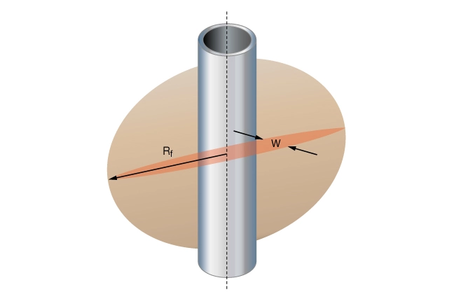
The maximum width at the center point of the wellbore is given as follows:

$W_{w,0} = 4.20\, \left( \dfrac{\mu \, q_i \, x_f}{E'} \right)^{\frac{1}{4}}$

and the average fracture width is

$\overline{w} = 0.533\, W_{w,0}$

Comparison of 2-D Models

A comparison of the PKN and KGD width equations shows that all parameters being equal, plots of fracture width versus fracture extent for the PKN and KGD models cross one another (Figure 4).

Comparison of relationship between fracture width and fracture length for KGD and PKN models, Hydraulic Fracturing, Fracturing fluids types, Fracture geometry, Frac job design, Hydraulic fracturing techniques, Fracture propagation, Fracking equipment, Fracturing fluid composition, Hydraulic fracturing explained, Fracking techniques, Hydraulic fracturing process, Hydraulic Fracturing, Fracking, Shale Gas Extraction, Fracture Stimulation, Fracturing Fluids, Proppants, Unconventional Oil and Gas, Hydraulic Fracturing Process, Frac Jobs, Fracture Network, Fracture Propagation, Horizontal Drilling, Hydraulic Fracturing Wells, Frac Sand, Well Stimulation, Shale Formation, Fracture Fluids, Fracture Treatment, Fracture Pressure, Reservoir Stimulation, Fracture Design, Fracture Width, Fracture Monitoring, Fracture Optimization, Fracture Mechanics — **Figure 4**: Comparison of relationship between fracture width and fracture length for KGD and PKN models

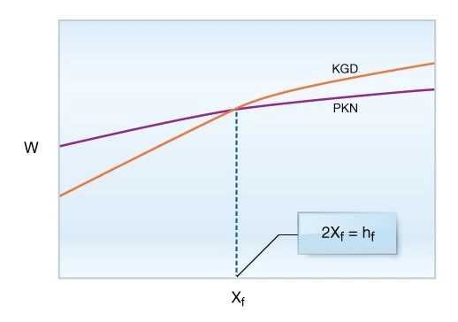
At smaller fracture lengths, the PKN width equation predicts larger width. The crossover occurs approximately at the point at which a “square fracture” has been created—the fracture height $(h_f)$ is equal to the total length of the fracture (2 times the fracture half-length or $2\, x_f$ ). While this fact has been used to argue for one or the other equation, the truth is that the physical assumptions behind the KGD equation are more realistic for small fracture extent situations. For larger fracture extents, however, the PKN width equation is physically more reasonable.

These equations relate fracture width and extent. Thus, if we know the fracture volume, we can use one or the other of these width equations to obtain the fracture dimensions. In the particular case of negligible leakoff, the fracture volume contains all of the fluid injected and is simply the injection rate multiplied by the injection time. Using this fact, we can derive the time behavior of a propagating fracture for the no-leakoff case, as summarized for the PKN, KGD, and radial models in Table 1.

Table 1: Equations relating fracture extent, width, and net pressure for three different 2-D hydraulic fracture models
	PKN	KGD	Radial
Extent	$x_f = 0.572\, \left( \frac{q_i^3\, E'}{\mu\, h_f^4} \right)^{\frac{1}{5}}\, t^{\frac{4}{5}}$ (original PK constant 0.524)	$x_f = 0.539\, \left( \frac{q_i^3\, E'}{\mu\, h_f^3} \right)^{\frac{1}{6}}\, t^{\frac{2}{3}}$	$R_f = 0.572\, \left( \frac{q_i^3\, E'}{\mu} \right)^{\frac{1}{9}}\, t^{\frac{4}{9}}$
Width	$\overline{w} = 1.75\, \left( \frac{q_i^2\, \mu}{E'\, h_f} \right)^{\frac{1}{5}}\, t^{\frac{1}{5}}$ (original PK constant 1.91)	$\overline{w} = 1.85\, \left( \frac{q_i^3\, \mu}{E'\, h_f^3} \right)^{\frac{1}{6}}\, t^{\frac{1}{3}}$	$\overline{w} = 1.95\, \left( \frac{q_i^3\, \mu ^2}{E'^2} \right)^{\frac{1}{9}}\, t^{\frac{1}{9}}$
Net Pressure	$p_{n,w} = 1.39\, \left( \frac{E'^4\, \mu \, q_i^2}{h_f^6} \right)^{\frac{1}{5}}\, t^{\frac{1}{5}}$ (original PK constant 1.52)	$p_{n,w} = 1.09\, \left( E'^2\, \mu \right)^{\frac{1}{3}}\, t^{\left( -\frac{1}{3} \right)}$	$p_{n,w} = 2.51\, \left( E'^2\, \mu \right)^{\frac{1}{3}}\, t^{\left( -\frac{1}{3} \right)}$
$\boldsymbol{\alpha}$	4/5	2/3	8/9
$\boldsymbol{k}$	1.415	1.478	1.377
$\mathrm{W_{w,0}} =$ maximum fracture width at center point of wellbore $\boldsymbol{E'} =$ Young’s Modulus (modulus of elasticity of rock) $\boldsymbol{q_i} =$ injection rate $\boldsymbol{\mu} =$ viscosity of injected fluid $\boldsymbol{x_f} =$ fracture half length $\boldsymbol{h_f} =$ fracture height $\boldsymbol{t} =$ pumping time $\boldsymbol{p_{n,w}} =$ net pressure

While the PKN model predicts an increasing treating pressure curve with pumping time based on the time exponent, the other two models predict decreasing pressure profiles. In addition, the PKN model implies that the net pressure is higher if the injection rate is larger. The other two models predict a net pressure varying with time independently of the injection rate, and therefore they are of limited practical use for pressure related analyses.

While it is not valid in general to assume that leakoff is negligible and that the entire volume of fluid injected determines the fracture dimensions, we can combine a particular width equation with material balance relations based on fluid leakoff and obtain a closed design model.

Other Processes Controlling Fracture Extension

Based on the present understanding of fracture propagation, in most cases simple two-dimensional models predict faster fracture propagation than actually occurs in the formation; tip propagation is usually impeded. This means higher-than-zero net pressure at the tip, because there is intensive energy dissipation in the near-tip area. Several attempts have been made to incorporate this tip phenomenon into fracture propagation models. One reasonable approach is to introduce an apparent fracture toughness that increases with the size of the fracture. Other approaches include a controlling relationship for the propagation velocity incorporating some additional mechanical property of the formation.

In principle, the lateral and vertical propagation of the fracture is subjected to the same mechanical laws. The substantial difference is that the fracture tip meets the same minimum stress during lateral propagation, while the vertical tip is likely to cross several layers with different material properties and stress states.

The equilibrium height concept (Simonson, et al., 1978) provides a simple and reasonable method of calculating fracture height if there is a sharp stress contrast between the target layer and the overburden and underburden strata. If the minimum horizontal stress is considerably larger in the over- and under-burden layers–for instance, by several hundred psi–we may assume that the fracture height is determined by the requirement of reaching the critical stress intensity factor at both the top and bottom tips. This requirement of equilibrium poses two constraints, and so the two penetrations can be obtained solving a system of two nonlinear equations. The solution can be plotted as a height-map, indicating what fracture height will be reached at a given treating pressure (Figure 5).

Fracture height map showing upper and lower fracture tip location as a function of treating pressure for a producing formation over and underlain by strata with different stress profiles, Hydraulic Fracturing, Fracturing fluids types, Fracture geometry, Frac job design, Hydraulic fracturing techniques, Fracture propagation, Fracking equipment, Fracturing fluid composition, Hydraulic fracturing explained, Fracking techniques, Hydraulic fracturing process, Hydraulic Fracturing, Fracking, Shale Gas Extraction, Fracture Stimulation, Fracturing Fluids, Proppants, Unconventional Oil and Gas, Hydraulic Fracturing Process, Frac Jobs, Fracture Network, Fracture Propagation, Horizontal Drilling, Hydraulic Fracturing Wells, Frac Sand, Well Stimulation, Shale Formation, Fracture Fluids, Fracture Treatment, Fracture Pressure, Reservoir Stimulation, Fracture Design, Fracture Width, Fracture Monitoring, Fracture Optimization, Fracture Mechanics — **Figure 5**: Fracture height map showing upper and lower fracture tip location as a function of treating pressure for a producing formation over and underlain by strata with different stress profiles

The dashed line is a second, unstable solution to the system of equations. Height-maps are advantageous for selecting the fracture heights to be used in simple two-dimensional design models. They also help us determine a treatment pressure limit (if, for instance, we must avoid fracturing into a water zone).

Three-Dimensional Models

Three-dimensional models have been developed to comprehensively model the creation of hydraulic fractures, fully accounting for fluid leakoff, two-phase and non-Newtonian flow behavior, heat transfer, proppant transport, wellbore hydraulics, PVT and rheological characteristics of both reservoir and fracturing fluids, and other factors. As with any complex model, the sensitivity to variations in the accuracy of the various required inputs may exceed the availability of good, representative data for these inputs. Nevertheless, these models are often used as the basis of treatment design programs offered by many hydraulic fracture stimulation service companies.