Applications of Geomechanics | What is the use of geomechanics?

30 minutes read

Learning Objectives

After completing this topic “Applications of Geomechanics“, you will be able to:

Relate geomechanical concepts to drilling applications.
Explain the completion application of sanding and potential risks that are involved.
Describe the completion application of hydraulic fracturing and the potential risks that are involved.
Recognize the completions differences in a horizontal well.
Use various geomechanics elements to create a coupled geomechanics model.

Introduction to Geomechanical Applications

This topic introduces geomechanics data and modeling applications used in the petroleum industry. Many of the applications listed in Table 1 require, as input, a majority of Mechanical Earth Model components.

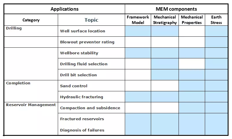
MEM Components Associated with Common Applications of Geomechanics Data and Modeling, Geomechanics, Applications of geomechanics — **Table 1:** MEM Components Associated with Common Applications of Geomechanics Data and Modeling

This course addresses geomechanics applications for the life of a field, with particular focus on the drilling and completion phases of field development.

Drilling applications include pre-drill planning and while-drilling wellbore stability management.
Completion applications include sanding risk analysis, completion design, and hydraulic fracturing stimulation planning and design.

The recurring theme throughout drilling and completion operations is the elastic stress concentration around a cylindrical opening in a stressed earth. This concept is central to understanding the mechanics of wellbore instability, sand production, and hydraulic fracturing.

Aspects of reservoir management such as compaction, subsidence, and fractured reservoirs are discussed. Finally, we outline a workflow for diagnosing operational failures including unplanned events that contribute to significant cost overruns such as lost-in-hole LWD tools, wellbore instability, production wells filling up with sand, and reservoir stimulations that fracture out of zone.

Drilling Applications

Geomechanics plays a role in drilling operations from pre-drill well planning to wellbore stability support while drilling. Drilling applications differ from completion applications in that drilling spans thousands of meters of depth and a wide range of rock types, whereas completions are restricted to reservoir intervals with few shale beds. Fortunately for the geomechanics team, the mechanical earth model (MEM) in the overburden can be less precise than it needs to be in the reservoir, where more data are available to calibrate it.

Mechanical Wellbore Stability

A practical definition of a stable wellbore is one that is drilled and cased in the reservoir without incident or cost overruns. There are two main causes of wellbore instability: mechanical failure of the rock due to drilling-induced stresses and wellbore deformation due to chemical reaction of rocks with the drilling fluids. Sometimes both occur. Chemical instability is the domain of the geochemist and drilling fluids specialist and it is not addressed here. The geomechanics focuses on predicting and managing rock mechanical failure. Two primary sources of mechanical instability are:

Deformation of intact rock
Destabilization of pre-existing planes of weakness

Wellbore stability studies typically address deformation of intact rock first, followed by destabilization of pre-existing planes of weakness.

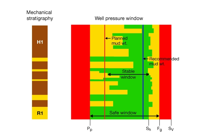
Specifying the safe and stable well pressure is important for drilling safely and within budget. Drillers need to know the safe wellbore pressure profile along a proposed well path before drilling can begin. The safe-pressure profile is bounded by pore pressure below and the fracture pressure above. Drilling with well pressure between these two limits will prevent a blowout but not wellbore instability.

The stable well pressure profile has a narrower pressure range. Typical drilling engineering places the low-pressure limit at the well pressure to prevent shear failure of intact rock, and the upper limit at the fracture pressure (the pressure at which a hydraulic fracture initiates at the wellbore surface). A more appropriate approach places the upper limit equal to the least principal stress magnitude, generally $S_h$ .

Figure 1 illustrates the concepts of safe and stable mud pressure ranges. Schematic diagrams of wellbore cross-sections illustrate natural and induced structures that both define the pressure window and affect drilling operations.

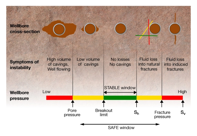
Examples of mud pressures ranges, Applications of geomechanics, Geomechanics, geomechanics — **Figure 1**: Examples of mud pressures ranges

Severe hole enlargement and high volume of solids production, or cavings, can result in drilling problems when wellbore pressure is near pore pressure and below stable. At the other end of the window, fluid loss into natural or induced hydraulic fractures can lead to a well blowout such as the Macondo disaster in the Gulf of Mexico.

Within the stable window, breakouts and losses do not occur. Drilling with well pressures in the yellow ranges is more risky. On the low pressure side, the risk is hole enlargement and solids production; on the high pressure side, the risk is fluid loss into natural fractures.

This diagram is limited to a specific depth in a well corresponding to a specific set of rock mechanical properties and earth stresses. The task for the geomechanics team is to estimate the stress and strength variations along a proposed well path so that the safe and stable well pressure window can be calculated for every depth interval. In some intervals there is no stable window and rock failure is unavoidable.

Mechanical wellbore stability is achieved by managing ΔP, the difference between wellbore pressure and pore pressure:

$\Delta P = P_{well} - P_p$

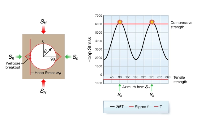
The following analysis illustrates how well pressure is used to manage wellbore stability. The wellbore surface can fail if the hoop stress, $\sigma _{\theta}$ , exceeds the formation’s tensile strength or its shear strength. The elastic hoop stress is calculated as a function of azimuth around the wellbore given the magnitude of pore pressure, and the maximum and minimum horizontal principal stresses $S_H$ and $S_h$ , respectively. In terms of effective stresses, $\sigma _{H}$ and $\sigma _{h}$ , the hoop stress is:

$\sigma _{\theta} = (\sigma _{H} + \sigma _{h}) - 2(\sigma _{H} + \sigma _{h})\cos 2\theta - \Delta P$

where $\theta$ is measured clockwise from the azimuth of the maximum horizontal stress.

This key equation explains how mud pressure is used to manage mechanical wellbore stability. For the safe and stable mud window, $\Delta P$ is positive. Therefore, raising the well pressure reduces hoop stress, and lowering the well pressure increases hoop stress.

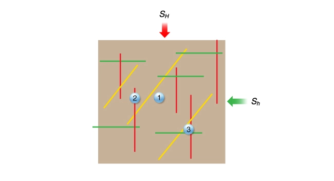
Figure 2 illustrates three hypothetical wells drilled in a naturally fractured formation. Assume these fractures are permeable and un-cemented and that the rock strength and earth stresses have been determined.

Three hypothetical wells in a naturally fractured formation, Applications of geomechanics, Geomechanics, geomechanics — **Figure 2**: Three hypothetical wells in a naturally fractured formation

How Mud Pressure Affects Wellbore Stability

First, consider well #1 that does not intersect natural fractures.

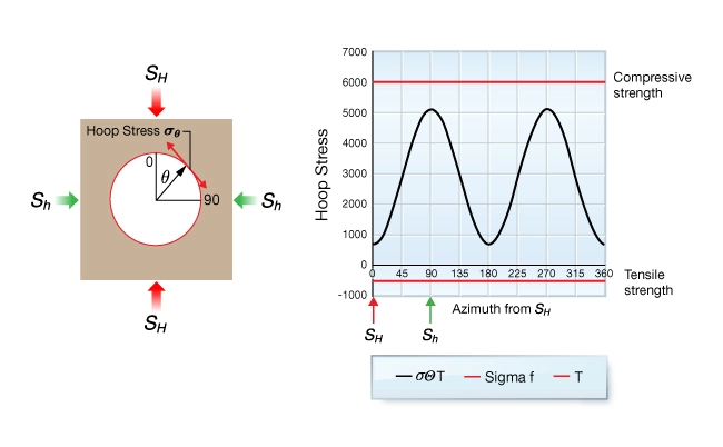
Figure 3 shows an example of well #1 where $\Delta P$ is optimal. At left is a cross-section of the well, and at right is the variation of hoop stress (black curve) as a function of azimuth around the well.

Well # 1 where ΔP-optimal is optimal, Applications of geomechanics, Geomechanics, geomechanics — **Figure 3**: Well # 1 where $\Delta P$ is optimal

The amplitude of stress variation is governed by the difference between $S_H$ and $S_h$ . If the horizontal stresses were equal, hoop stress would be the same at all azimuths and plot as a horizontal line. The effect of changing the well pressure is to shift the hoop stress curve up or down by the amount of $\Delta P_{well}$ . Note that the hoop stress does not intersect the strength curves anywhere on the wellbore surface. In the context of the wellbore pressure window this is a stable mud pressure which plots in the green region.

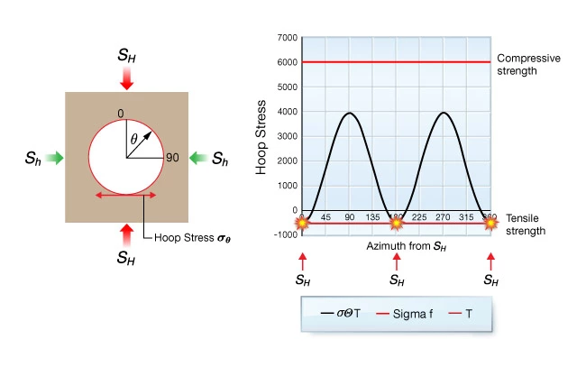
Figure 4 shows an example of well #1 where the wellbore pressure is too high, causing hydraulic fractures to initiate at the azimuth of $S_H$ . The only difference between Figure 4 and Figure 3 is that the well pressure was increased. Notice that the hoop stress now equals the tensile strength of the rock at ($ \theta $=0 degrees and 180 degrees). If the well pressure were to be reduced, the hoop stress would increase by the same amount at all azimuths.

Well # 1 where ΔP-optimal is too high, Applications of geomechanics, Geomechanics, geomechanics — **Figure 4**: Well # 1 where $\Delta P$ is too high

Figure 5 illustrates what happens when the well pressure in well #1 is too low. The hoop stress equals the rock’s compressive strength at the azimuth of $S_h$ , causing shear failure of the wellbore surface (such as wellbore breakouts). This corresponds to the breakout limit at the low pressure side of the stable region of the wellbore pressure window.

Well # 1 where ΔP-optimal is too low, Applications of geomechanics, geomechanics — **Figure 5**: Well # 1 where $\Delta P$ is too low

Well #2 and Well #3 show how natural fractures can affect the maximum well pressure (Figure 6). Well #2 intersects a natural fracture aligned with the maximum horizontal stress. The normal stress acting on this fracture is equal in magnitude to the least horizontal stress. If the well pressure is greater than the least horizontal stress ( $P_{well} \geq Sh$ ), the fracture dilates and the well starts to loose fluid.

Well #3 intersects all three fracture sets. However, fractures aligned with $S_H$ will still open first because the normal stress on the yellow and green fractures is much greater than $S_h$ .

Three hypothetical wells in a naturally fractured formation, Applications of geomechanics, geomechanics — **Figure 6**: Three hypothetical wells in a naturally fractured formation

The azimuthal variation of normal stress on vertical natural fractures can be calculated by:

$S_n = \dfrac{1}{2} (S_H + S_h) + \dfrac{1}{2} (S_H - S_h) \cos(2\theta)$

Figure 7 shows an example of fracture normal stress as a function of angle from the direction of $S_H$ . At $\theta$ =0, the normal stress is $S_h$ , at $\theta$ =90, it is $S_H$ . Colored dots on the graph indicate the normal stress on the fractures. In addition to the formation breakdown pressure, the opening pressures of natural fractures can limit the maximum mud pressure used to drill a well. Therefore, the magnitude of the least horizontal stress is often used as a conservative upper bound pressure for the stable mud weight window.

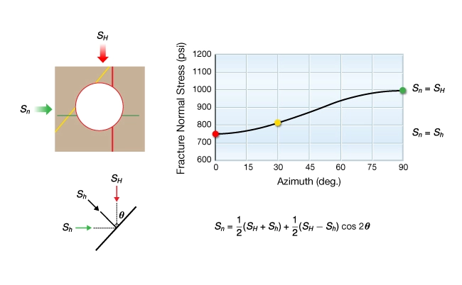
Example of normal stress as a function of angle, Applications of geomechanics, geomechanics — **Figure 7**: Example of normal stress as a function of angle

Drilling fluid losses will develop when the well pressure exceeds the fracture normal stress. The least fracture normal stress is equal to the magnitude of $S_h ( \theta = 0)$ . This corresponds to the right edge of the stable mud pressure window.

Stability of Deviated Wells

Few wells drilled today are vertical. Offshore fields are developed from fixed or floating drilling platforms using multiple deviated and extended reach wells to access reservoirs. The stability of arbitrary well trajectories must be modeled numerically. However, it is straightforward to analyze the stability of vertical and horizontal wells drilled in the direction of the three principal stresses. This situation applies to most shale-gas reservoirs which are completed from horizontal wells.

To illustrate, consider the relative stability of wells aligned with the three principal stresses in a normal faulting stress regime and where $S_H$ is slightly less than $S_V$ as we see in Figure 8.

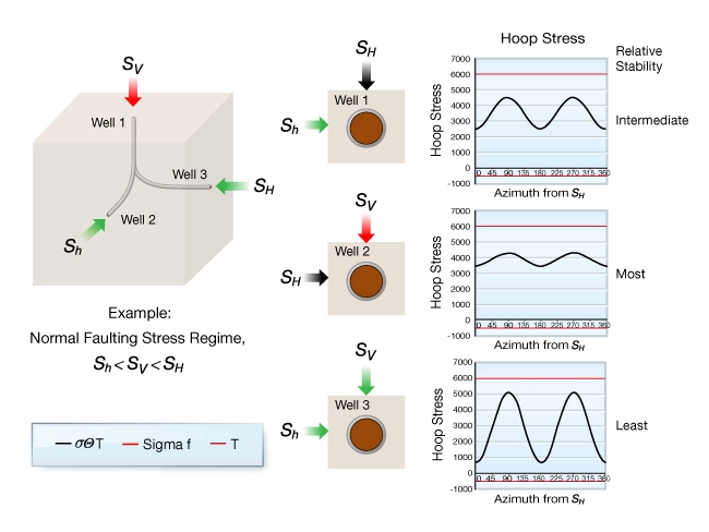
Stability of vertical and horizontal wellbores in relation to the three principle stresses, Applications of geomechanics, geomechanics — **Figure 8**: Stability of vertical and horizontal wellbores in relation to the three principle stresses

Assume that a stable mud pressure exists. The relative stability of different trajectories are determined by analyzing wellbore stress concentrations. The most stable trajectory is the one where the hoop stress variation around the borehole is minimized. That is, when the difference between the principal stresses, in the plane normal to the axis of the well, is the smallest. Figure 8 shows that the least stable well is a horizontal well drilled toward the intermediate principal stress $S_H$ . The most stable well is a horizontal well drilled toward $S_h$ . A vertical well is intermediate between these extremes.

For any given stress regime, the well with the greatest risk of mechanical wellbore instability is one drilled in the direction of the intermediate principal stress. Knowledge of the relative magnitudes of the all three principal stresses is needed to rank the relative stability of the other two directions. Note that even the well with the highest relative risk of instability can be drilled if a suitable well pressure can be found.

Drilling Planning

The geomechanics team normally gets involved once the exploration department has identified a drilling prospect. Upon budget approval, the exploration department supplies the drilling department with a subsurface target. The drilling department must then prepare a detailed drilling program and cost estimate for testing the rocks at the target location. Geomechanics input is necessary to determine:

Surface location and well trajectory
Blowout preventer (BOP) rating
Number of casing strings
Casing setting depth
Drill bit selection
Wellbore stability forecast

Surface Location

The optimal surface location minimizes drilling problems and cost. For example, a vertical well can use fewer strings of casing and less drilling fluid but may not be optimally located for wellbore stability. Choosing an optimal location requires an earth stress analysis, including pore pressure, a review of potential drilling hazards, and a wellbore stability analysis along a variety of potential well paths. A structural interpretation of 3D seismic identifies the main drilling hazards such as the location of faults and fracture zones and their potential to contribute to mechanical wellbore instability. A pore pressure analysis based on seismic compressional wave velocity will help define the spatial variations of pore pressure and the minimum pressure along the proposed well path; the upper bound on the mud pressure window will be poorly constrained, however.

BOP Size

The working pressure of the BOP must exceed the maximum pore pressure that the well may encounter. This is best obtained by joint analysis of pore pressure predictions based on basin modeling, offset well data, and most importantly, pore pressure modeling based on seismic velocity.

Casing Points

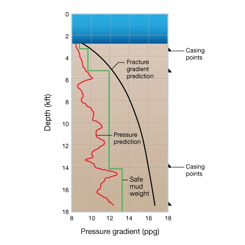
The number of casing strings and their setting depths is determined by the pore pressure and fracture gradient as a function of depth. Casing points are selected so that the maximum mud pressure at the base of a hole section does not exceed the fracture pressure at the last casing shoe. Figure 9 illustrates this concept for a deepwater exploration well.

Drill Bit Selection

Formation abrasiveness and compressive strength are two rock properties used for drill bit selection. Abrasiveness is related to the hardness of the rock-forming minerals which are captured in the mechanical stratigraphy. Rock strength and earth stresses contribute to the selection process in light of offset well drilling performance data. Some bit selection algorithms call for unconfined compressive strength (UCS); others for the confined compressive strength (CCS). Rock strength is modeled as:

$\sigma _f = UCS + \sigma _c \tan^2 \left( \dfrac{\phi}{2} + \dfrac{\pi}{4} \right) = CCS$

The total expression is referred to as the confined compressive strength or CCS. A quantitative estimate of the range of strength expected over a depth interval helps select the optimal bit for the section.

Wellbore Stability Forecast

A wellbore stability forecast has three parts:

A mechanical stratigraphy graphic showing the grain-support and clay-support facies
A wellbore pressure window
A list of potential drilling hazards and risks and recommendations for remedial action

Figure 10 shows a schematic of a wellbore stability forecast. Drilling fluids are selected so they do not react chemically with clay minerals identified in the stratigraphic section. The wellbore stability forecast predicts either breakouts or fluid losses when drilling with pressures outside of the stable window. Known drilling hazards and potential risks are identified along with recommended remedial action. The vertical red line represents the well pressure corresponding to a specific drilling fluid density. The vertical blue line is the recommended pressure to drill this section of hole.