Related Articles


Reservoir Geomechanics
Reservoir geomechanics focuses on deformation induced by changes in pressure in the entire reservoir. Decreasing reservoir pressure can lead to sanding, reservoir compaction, and decreased permeability in naturally fractured reservoirs. Increases in reservoir pressure can lead to fault activation and casing deformation, and increased reservoir permeability. The role of geomechanics is to evaluate the impact of reservoir pressure change on reservoir deformation and to help manage its effects on field operations.
Geology and geophysics play significant roles in reservoir geomechanics because of the need to predict and map spatial variations of rock properties in the inter-well region. Spatial variations of rock mechanical properties affect predictions of rock strength and numerical computation of stresses in each geocell of a 3D geomechanical model. Knowledge of spatial variations affects decisions on the surface location and trajectory of wells and where to expect wellbore instability, solids production, and fault movement.
Coupled Geomechanics Modeling
As the complexity and cost of reservoir development increases, the industry is employing coupled geomechanics modeling to predict where and when deformation will occur. Reservoir simulators predict the change in reservoir pressure as a result of production; adding the time dimension makes a 3D geomechanical model 4D. Calculations are then used to interpret 4D seismic surveys, to predict when wells might be lost due to compaction or fault movement, and to identify high-risk and low-risk wells to drill as a function of time.
The process begins by constructing a 3D geomechanical model of the reservoir, the surrounding formations and one or more wells. Each geocell in the model is populated with rock mechanical parameters. Geocells in the reservoir also contain the reservoir parameters. The model contains the input parameters required by a geomechanics simulator and a reservoir simulator. An iteratively coupled approach to reservoir geomechanics modeling. Figure 1
Reservoir Geomechanics Modeling
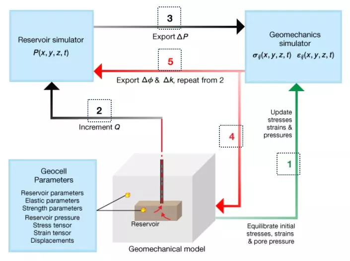
1. The geomechanics simulator computes the equilibrated state of stress and strain given the boundary conditions, initial pore pressure and the initial rock properties.
2. The reservoir simulator computes a change in reservoir pressure caused by an increment of production.
3. The changes in reservoir pressure are exported to the geomechanics simulator.
4. The geomechanics simulator then recalculates the stress and strain fields given the new reservoir pressure. Changes of stress and strain cause changes of porosity and permeability and these are exported to reservoir simulator.
5. Pass changes in porosity and permeability to the reservoir simulator.
This process is repeated from Step 2, until the production schedule has been fully simulated. The resulting calculations reveal the time evolution of pressure and rock deformation over the entire 3D volume, not just in the reservoir.
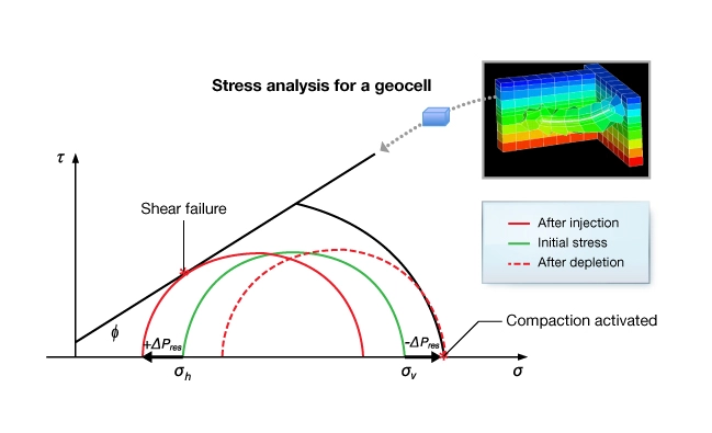
Figure 2 illustrates how a geocell may deform in response to a coupled reservoir-geomechanical calculation. A geocellular model containing a deviated wellbore and a Mohr stability diagram represents the state of stress in one of the geocells. The green Mohr’s circle represents the initial state of stress, that is, before the well is put on production. Once the well has been on production the reservoir pressure drops. If it drops enough, the effective stress may satisfy the criterion for compaction (dashed red line). If a sufficient number of the geocells surrounding the well satisfy the criterion, the casing can fail in shear, resulting in a loss of production from the well. Conversely, if fluid pressure increases by injecting fluids, the geocell may fail either by mode 1 fracturing or by activating slip on pre-existing fractures or faults. Shear failure is depicted by the solid red circle. This type of model is used to manage reservoir pressure over time.
Fractured Shale Reservoirs
As a final example for reservoir geomechanics, consider a fractured shale-gas reservoir. A change in reservoir pressure affects permeability as well as the potential for slip on suitably oriented fractures and faults.
Pressure Effects in Fractured Shale Reservoirs
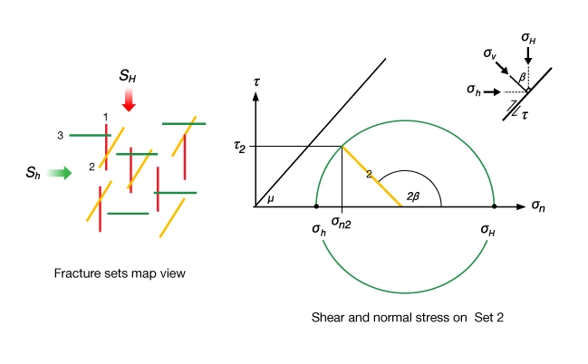
Figure 3 shows a map view of a reservoir containing three fracture sets in relation to the far-field horizontal stresses  and
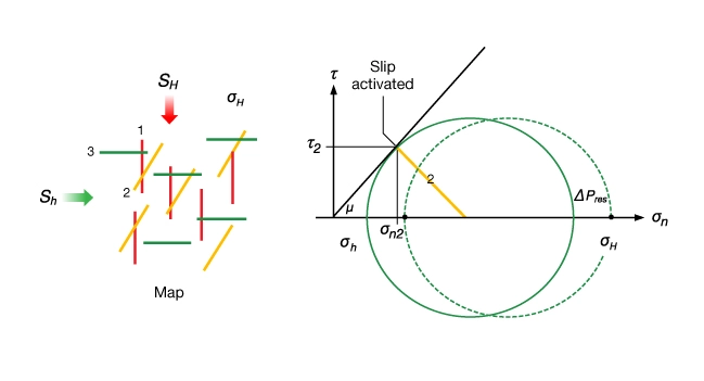
and  . Assume that the state of stress is uniform throughout the reservoir, and the fracture compressibility is the same for all fractures. (In reality, fracture compressibility is likely to vary with each fracture set.) To the right is a Mohr’s circle representation of the initial state of stress on fracture set 2. The shear and effective normal stresses are shown by the dotted gray lines. When reservoir pressure increases, effective normal stresses decrease and the Mohr’s circle shifts to the left. When reservoir pressure increases enough, the shear stress on set 2 fractures satisfies the slip criterion and shear displacement occurs along the fracture plane.
When the displacement happens fast enough, a microseismic event is triggered. This is what often happens when naturally-fractured shale reservoirs are stimulated by hydraulic fracturing (Figure 4). The dotted green circle represents the initial state of stress on fracture set 2. The solid green circle shows the state of stress after fluid pressure increased enough to cause slip on the fracture plane.
Consider how a change in reservoir pressure affects fracture permeability. Assuming fracture permeability obeys the parallel plate flow law, permeability varies as the square of fracture aperture  :
:

Since fracture aperture is a function of the effective normal stress on the fracture, changing reservoir pressure changes fracture permeability (Waters et al., 2011). Figure 5 shows schematically how fracture permeability varies with effective normal stress. The map view (left) shows the fracture orientations relative to the horizontal stresses. The graph shows how permeability varies with changes in effective normal stress. Notice how fracture orientation relative to the stress affects the initial permeability in wells as changes in reservoir pressure can change permeability.
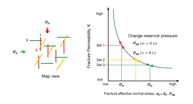
Anisotropic earth stresses impart a permeability anisotropy to the reservoir such that:  . A uniform change in reservoir pressure changes the permeability of all fracture sets, but by different amounts for each set, depending upon the initial fracture normal stress (see colored arrows). Thus a change in reservoir pressure changes both permeability and permeability anisotropy (Brown, 1989).
Diagnosis of Failures
Often, geomechanics is not involved in oilfield operations until there is a problem. The challenge is to figure out what happened and to recommend remedial action. The sequential workflow for diagnosing the root cause of a geomechanics problem is to:
- Review the engineering basis of design.
- Review operational activities leading up to the event.
- Determine if the deformation (failure) was caused by unexpected stresses, rock strength, geologic structure, or failure to follow the design.
- Recommend changes in design, operational practices, or both.
Ideally, a mechanical earth model (MEM) is developed early in the life of a field, and is updated as new information becomes available. This proactive approach enables the diagnosis and recommendations to be completed relatively quickly and improves the effectiveness of field development planning. In a reactive approach, the MEM must be developed before step three can be completed. This can take weeks to months depending on the complexity of the problem and the availability of existing data.