Earth Stress | What is Earth stress?

50 minutes read

Stress-directions-from-shear-wave-anisotropy

Contents

Learning Objectives Introduction to Earth Stress Stress Notation Contemporary Stress Reference States of Stress Lithostatic Pressure Vertical Stress Hydrostatic Pressure Specifying an Earth Stress Regime

Learning Objectives

After completing this topic “Earth Stress”, you will be able to:

Define the different reference states of stress.
Differentiate contemporary stress from paleo stress.
Compare and contrast different constraints for determining contemporary stress.
Differentiate borehole imaging tools.
Describe the factors influencing horizontal stress in sedimentary basins.
Summarize the models for determining horizontal stress.

Introduction to Earth Stress

Earth stress drives rock deformation in the subsurface. Quantitative information about the current state of stress is needed to understand the cause of rock deformation, and to prevent or manage it. Until the mid-1950s, it was common for petroleum engineers to assume that the in-situ stress field was lithostatic and equal in magnitude to the weight of the overburden. However, Hubbert and Willis (1957) noted that geologic faults could not develop in a state of lithostatic stress. They also observed that hydraulic fracturing in reservoir rocks occurred at pressures well below the magnitude of the overburden stress. They argued that there must be three unequal principal stresses and that one is significantly less than the overburden stress.

This course introduces methods for characterizing the contemporary state of stress in sedimentary rocks. We begin by presenting background information that is helpful for understanding the stress modeling workflow. This includes distinguishing contemporary stress and paleo stress, defining common reference states of stress and defining stress regimes. With this background, we will then step through the process of characterizing the state of stress for a specific geographic location. Developing new information about in situ stress evolves in this sequence:

Establish regional constraints on the contemporary stress regime.
Make borehole measurements which provide data to model the vertical profile of stress.
Calibrate the stress model.

In addition, we will examine the natural variability of horizontal stress measured in sedimentary rocks. Pore pressure, lithology, and diagenesis affect variation of stress magnitudes within and between sedimentary basins. Stress models can replicate this natural variability.

This workflow results in a quantitative description of the contemporary stress that has value for predicting the life of a field. The stress model may be used to supply inputs to forecast wellbore stability, design reservoir completions, or to diagnose the causes for reservoir deformation.

Stress Notation

In many practical situations, as well as in this course, it is assumed that the vertical stress is a principal stress. When this is true, quantities that may completely specify the state of stress at a point include: three principal total-stress magnitudes ( $S_V$ , $S_h$ , [/latex] S_H [/latex]), pore pressure ( $P_P$ ), and the azimuth of one of the horizontal stresses ( $S_h$ , or $S_H$ ). As stated below, each notation should be clearly defined before any calculations are made.

The effective stress tensor, or the relationship between stress and pore pressure, in principal coordinates is expressed as:

$\sigma_{ij} = \begin{bmatrix} S_{11} - P_P & & \\ & S_{22} - P_P & \\ & &S_{33} - P_P \end{bmatrix}$

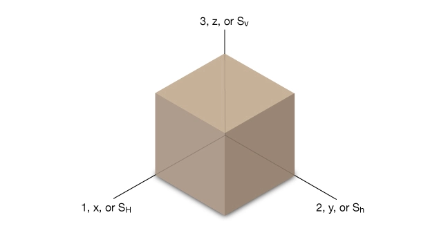
Geomechanics nomenclature can be confusing because subscripts can refer either to coordinate axes (1, 2, 3 or $x$ , $y$ , $z$ ), or the relative magnitudes of the principal stresses (1, 2, 3). To minimize confusion, the following convention is employed. Assuming that the vertical stress is a principal stress and that its relative magnitude is unknown, it is convenient to write the effective stress tensor as:

$\sigma = \begin{bmatrix} S_{H} - P_p & & \\ & S_{h} - P_p & \\ & &S_{v} - P_p \end{bmatrix}$

Where:

$\sigma$ represents effective stress tensor

$S$ represents total stress such that: $S_H$ is the greatest horizontal principal stress, acting along the $x$ or 1 axis

$S_h$ is the least horizontal principal stress, acting along the $y$ or 2 axis

$S_v$ is the vertical principal stress, acting along the $z$ or 3 axis

$P_p$ is the pore pressure

Figure 1 explains the relationship between three subscripting conventions used in the discussion of principal stresses.

**Figure 1**: The three principle stresses

Contemporary Stress

Before attempting to characterize the contemporary state of stress, it helps to distinguish it from paleo-stress. Contemporary stress governs current rock deformation related to such phenomena as wellbore instability, the propagation of hydraulic fractures and active faulting. Paleo-stress, in contrast, is responsible for past rock deformation events such as the formation of folds, faults, and sedimentary basins. The paleo-stress regime associated with the Appalachian Mountains, for example, is very different from the contemporary one, whereas the San Andreas Fault evolved over millions of years in a stress regime similar to its contemporary one. Because of the complex loading and diagenetic history that rocks experience over geologic time, it is not possible to accurately predict the contemporary stress from first principles. The approach presented in this course is to calibrate models of stress using in-situ measurements and knowledge of how earth stresses vary naturally.

Reference States of Stress

When working with earth stresses it helps to have a frame of reference or a reference state of stress. Lithostatic pressure and hydrostatic pressure are examples of two reference states used frequently in earth stress analysis. Two others are the uniaxial strain and frictional equilibrium models. A reference state of stress allows one to readily distinguish between normal and abnormal stress levels and to recognize differences of stress from one location to another (Engelder, 1993).

Lithostatic Pressure

The simplest reference state is that of lithostatic pressure. Imagine that the outer 25 km of the earth consists of molten rock with bulk density $\rho _b$ . Lithostatic pressure, $L$ , is the force per unit area exerted by a vertical column of molten rock extending from the surface to depth $z$ :

$L = g\, \displaystyle \int _{\, 0} ^{\,z} \rho _b (z)\, \mathrm{d}z$

Where:

$g$ is the acceleration of gravity

$\rho _b$ is the bulk density of the molten rock

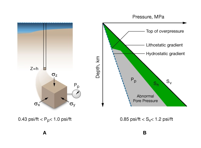
Lithostatic pressure is the same in all directions. A lithostatic gradient of 1 psi/ft or 22.6 MPa/km is a common reference state of stress (Figure 2).

diagram state of stress — **Figure 2**: Schematic diagram illustrating a common reference state of stress: (A) computation of hydrostatic pressure, lithostatic pressure, and vertical stress; (B) typical ranges for pore pressure, $P_p$ , least horizontal stress, $S_h$ and vertical stress, $S_v$

Shales are sometimes said to be in a state of lithostatic stress. The idea is that over geologic time, shale behaves like a liquid and the state of stress becomes lithostatic. As we see later in this discussion, this premise is generally false.

Vertical Stress

Vertical stress, $S_V$ , or overburden stress as it is often called, is a normal stress acting in the $z$ direction. It is the force per unit area at depth $z$ , due to the weight of the overlying vertical column of rock (Figure 2A):

$S_v = g\, \displaystyle \int _{\, 0} ^{\,z} \rho _b (z)\, \mathrm{d}z$

Vertical stress is a total stress so the effective vertical stress, $\sigma _v$ is defined as:

$\sigma _v = S_V - P_p$

Although they are numerically equivalent, it is important to distinguish vertical or overburden stress from lithostatic pressure. Stress implies that the rock has shear strength and that three principal stresses exist. Pressure, on the other hand, is isotropic, or equal in all directions.

As with lithostatic pressure, a vertical stress gradient of 1 psi/ft is a common reference state used in geosciences and the petroleum industry. Note that the vertical stress gradient is not constant but usually increases with depth. This effect is greatest in young offshore basins where gradients can be as low as 19 MPa/km near the surface and as much as 22.6 MPa/km or more at depth. In older basins the vertical stress gradient is less variable with depth and can be as high as 25 to 26 MPa/km.

Hydrostatic Pressure

Hydrostatic pressure is the force per unit area exerted by a column of fluid with density $ P_f $ extending from the surface to a depth $ z $ and computed as:

$P_f = g\, \displaystyle \int _{\, 0} ^{\,z} \rho _b \, \mathrm{d}z$

Hydrostatic pressure is the reference pressure used to define overpressure (Figure 2A).

Overpressure, or abnormal pressure, refers to pore pressure that exceeds the hydrostatic pressure of the native formation water. In virgin formations, pore pressure can vary from hydrostatic to nearly lithostatic (Figure 2B). In practice, formation pressures rarely reach lithostatic pressure because natural hydraulic fracturing releases some of the excess pressure (Engelder, 1993; Secor, 1969).

In this discussion, normal pore pressure ( $P_{pn}$ ) is defined as the hydrostatic pressure of fresh water, given by:

$P _{pn} = g\, \displaystyle \int _{\, 0} ^{\,z} \rho _b \, \mathrm{d}z$

Where:

$P_f =$ 1.0 g/cm³

the normal pore pressure gradient is 0.433 psi/ft or 10 MPa/km.

Figure 2 illustrates the concepts of hydrostatic and lithostatic reference states and how they are computed. An imaginary column of fluid-saturated rock is used to compute hydrostatic pressure, lithostatic pressures and vertical stress. Depth variations of these reference states are also shown. Gray shading indicates the domain where measurements of pore pressure, $P_p$ , would plot; green shading shows where measurements of the least horizontal stress, $S_h$ , would plot.

Specifying an Earth Stress Regime

In a poroelastic solid, the state of stress at a point is fully specified by three principal effective stress magnitudes and the orientation of the principal stress axes. In earth sciences and in geomechanics it is useful to speak of stress regimes rather than stress at a point. Clearly, it is impractical to measure stress at every point in the earth. However, it is practical to characterize the contemporary stress regime by specifying the relative ordering of principal stress magnitudes, the pore pressure gradient, and principal stress directions.

In regions of the earth where the stress regime is uniform, the relative ordering of the three principal stresses and stress direction changes little with depth or lateral position. For example, the state of stress or stress regime must be relatively homogeneous over great distances when geologic faults are created. Table 1 shows an example of the stress regime determined for the Cusiana field in Columbia. Establishing the stress regime constrains the state of stress at the shorter length scales that are characterized by geomechanical stress models.

Stress Component	Value psi/ft (MPa/km)	Relative Ordering
$S_V$	1.08 $\quad$ (24.4)	$S_2$
$P_p$	0.465 $\quad$ (10.5)
$S_h$	0.65-0.75 $\quad$ (14.7-17.0)	$S_3$
$S_H$	1.2-1.5 $\quad$ (27.4-33.9)	$S_1$
$S_H$ azimuth	N 53º W ± 11º

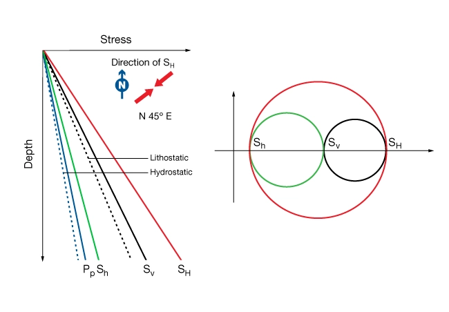
Table 1: Example of an Initial Stress Regime Determined for the Cusiana Field

Figure 3 is a graphical display of a stress regime. It shows the average gradients of the three principal stresses referenced to hydrostatic and lithostatic pressure (dotted lines, 10.1 MPa/km, and 22.6 MPa respectively). An inset map view shows the azimuth of the maximum horizontal stress. A Mohr’s circle representation of the stress regime is shown for reference.