Rock Mechanical Properties

31 minutes read

Laboratory Testing of Static and Elastic Properties

Laboratory testing plays two supporting roles in geomechanics.

The first is research into how intrinsic and extrinsic factors influence rock deformation. Laboratory testing helps to identify the intrinsic rock properties that govern a rock’s mechanical behavior and therefore which geophysical measurements may be used to measure them.
The second is calibration. Laboratory testing is also done to calibrate geophysical estimates of elastic and rock strength parameters when they are required for engineering design.

The pressure dependence is the main reason rock mechanical properties cannot be treated as constant and why laboratory testing is important. Sandstones, shales, and carbonates exhibit significantly different mechanical behavior and studies have demonstrated that, for any given lithology, porosity and clay content played a predictable role governing rock strength (Hoshino et al., 1972; Dobereiner and Freitas, 1986; Plumb et al., 1992; Plumb, 1994).

Triaxial Test Apparatus

The triaxial test is the most common method used to measure elastic and compressive strength parameters of rock. It is used to determine static and dynamic elastic parameters and to characterize rock failure criteria.

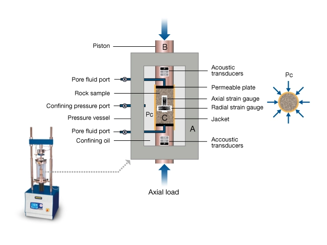
Figure 1 shows a schematic of the triaxial test apparatus. The main components are the pressure vessel (A), a piston that provides an axial load (B) to a cylindrical rock sample (C), and fluid ports (D). (The load frame and hydraulic systems are not shown.)

Schematic triaxial test apparatus, Rock mechanical properties, Geomechanics — **Figure 1**: Schematic of a triaxial test apparatus

The apparatus can apply independent control of axial load, $\sigma _{A}$ , radial confining pressure, $\sigma _r = P_c$ , and pore fluid pressure, $P_p$ . Despite the name, only two stresses are independent: the axial stress, $\sigma _A = \sigma _1$ , and the confining stress $P_c = \sigma _2 = \sigma _3$ .

Rock deformation is measured by gauges located inside the pressure vessel. Figure 1 shows axial and radial strain gauges. Other devices commonly used to measure deformation include linear variable differential transformers (LVDTs) and cantilevered gauges. In all cases the stress-strain curves are interpreted the same way.

Acoustic transducers, housed in the end caps, are used to measure compressional and shear wave velocity along the axis of the sample. Transmitters are in one end cap, receivers are in the other. Measurements may be made while the rock is deforming, or when it is in equilibrium at a particular state of stress. There can be two or three transducers in each end cap. One configuration has a P-wave and one S-wave transducer the other has a P-wave and two S-wave transducers polarized 90 degrees to each other. Two S-wave polarizations enable measurement of anisotropic elastic parameters.

The Triaxial Test

Triaxial tests typically employ one of three protocols:

One protocol provides rock parameters for a specific in-situ stress state.
A second protocol provides elastic properties and compressive strength over a range of confining pressures.
The third protocol, called a multi-stage test, is a hybrid of the first two.

Most tests are run under drained conditions at loading rates between 10⁻⁶ or 10⁻⁵ per second to prevent pore pressure gradients from developing in the sample.

In the first protocol the sample is loaded hydrostatically up to the desired confining pressure. The axial load is then increased either until the sample reaches a pre-defined deviatoric stress level or failure occurs. Mechanical properties are derived from the stress-strain curves thus obtained. This protocol is used when rock properties are needed for a specific engineering application such as hydraulic fracture design. It is less expensive but offers limited value for life of field applications.

The second protocol is the first protocol applied to a suite of samples, each tested at a different confining pressure. This is how the pressure dependence of mechanical properties is determined. Ideally there will be no significant variation of rock composition or texture among the test samples. This protocol is used to characterize a rock’s elastic parameters and failure criterion over a range of depths or production-induced changes of in-situ stress.

In a multi-stage test, a single rock sample is deformed over a range of confining pressures. The sample is loaded hydrostatically to the initial confining pressure, typically about 1-to-5 MPa. The axial load is increased until the sample reaches a predefined deviatoric stress level or its yield stress. At yield, the axial stress is stopped and the confining pressure is increased to the next programmed value and the process is repeated. Multi-stage tests are typically run at 3 to 5 times confining pressures. The test provides the pressure dependence on elastic parameters and a conservative estimate of compressive strength. A multi-stage test is used when core material is limited.

Static Elastic Properties

Elastic moduli characterize the rock’s response to stress, and are determined in triaxial cells under drained conditions. These are the parameters used in geomechanics calculations where rock strains exceed about 10⁻⁶.

Isotropic rock

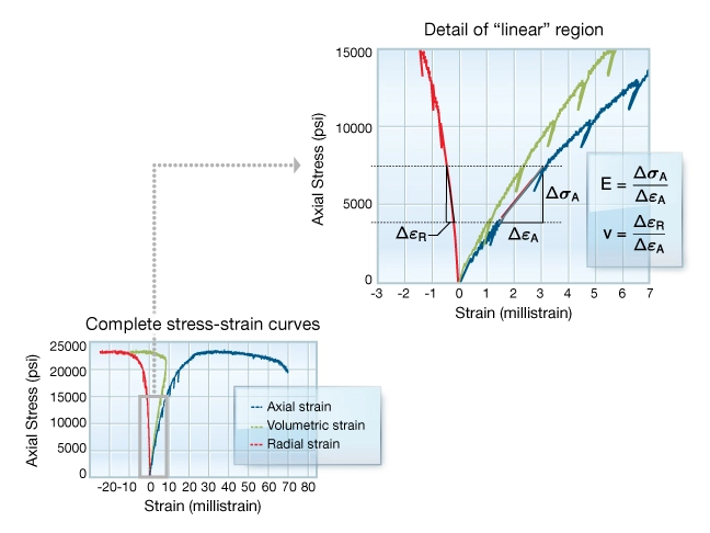
Two independent parameters are needed to characterize the elastic response of isotropic rocks at a particular confining pressure, and can be measured on a single sample of rock. Figure 2 illustrates three deformation curves recorded in a typical triaxial test plotted versus axial stress. They include an axial stress curve (blue), a radial strain curve (red), and a volumetric strain curve (green). The graph on the right shows the complete stress-strain curves. The gray shaded region indicates the linear portion of the curves where the static elastic parameters are computed. This region is expanded on the left. Referring to the figure on the left, note the interval of axial stress where Young’s modulus, $E$ , and Poisson’s ratio, $\nu$ , are computed. It is important that all the parameters are defined over the same interval of axial load. These are the elastic moduli reported in virtually all laboratory reports.

Shear modulus is not measured directly in a triaxial apparatus. But for isotropic rock, it can be computed from Young’s modulus and Poisson’s ratio:

$G _{stat} = \dfrac{E}{2 \, (1 + \nu)}$

Also in Figure 2 left, note the small subvertical portions of the deformation curves, spaced at regular strain intervals. These represent the rock’s response to small unload-reload stress cycles. Young’s modulus and Poisson’s ratio can be computed from such stress cycles over a range of axial loads. Compared to the primary loading curve, steeper slopes are evident for these stress cycles. This illustrates that elastic moduli depend upon the magnitude of stress change used to measure them. A similar effect is observed when comparing dynamic moduli to either of these static moduli.

Bulk modulus and bulk compressibility are obtained from deformations measured under hydrostatic stress. A hydrostatic test can be performed in a triaxial cell by using a controller to keep the axial stress and the confining pressures equal during loading as shown in Figure 3. The bulk modulus is computed from the slope of the $P$ vs. $\varepsilon _v$ curve in the linear portion of the loading curve. Non-recoverable mechanical compaction initiates at hydrostatic pressure, $P^*$ .

Schematic of the hydrostatic test apparatus (left) and a pressure vs. volume strain curve (right), Rock mechanical properties, Geomechanics — **Figure 3**: Schematic of the hydrostatic test apparatus (left) and a pressure vs. volume strain curve (right)

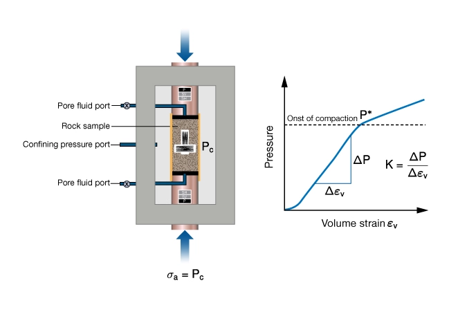
A variety of bulk moduli are defined for poroelastic materials. All can be obtained from a hydrostatic test depending on the way it is conducted (Table 1).

Table 1: Poroelastic Bulk Moduli Obtainable from a Hydrostatic Test
Modulus		Test conditions	Describes
Frame modulus	$K_f$	Jacketed, drained	Response of the solid frame
Bulk modulus	$K_B$	Jacketed, undrained	Response of the fluid+frame
Average bulk modulus of grains	$K_S$	Unjacketed	Average bulk modulus of rock forming grains in a poly-mineralic rock
Bulk modulus of the grains	$K_G$	Unjacketed	bulk modulus of rock forming grains in a mono-mineralic rock

These are parameters required by the Biot-Gassmann theory when calculating dry frame moduli from geophysical data. For further information about these tests and their interpretation, see Wang (2000).

Transversely Isotropic Rock

It is widely recognized that many shales are transversely isotropic (TI) materials. TI-V shale is one where the isotropic plane is horizontal and the axis of rotational symmetry is vertical. A TI-V material is characterized by five static stiffness parameters. The five parameters can be obtained from triaxial tests conducted on three core plugs (Figure 4). The plugs are cut perpendicular (A), parallel (B), and at 45 degrees (C) to the isotropic plane.

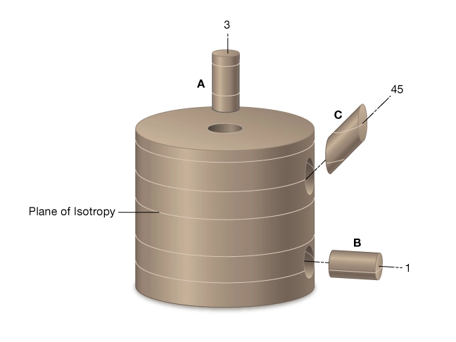
Table 2 provides the moduli obtained from deformations measured on each of the three core plugs.

Plug Identification	Experimental data
A	$E_3$ , $\nu_{31}$
B	$E_1$ , $\nu_{13}$ , $\nu_{12}$
C	$E_{45}$

Table 2: Correspondence Between the Orientation of Core Plugs and TI-V Parameters Determined from Them

Geophysicists and petrophysicists prefer to work in terms of the stiffness matrix. The stiffness matrix, $C$ , for a material with an axis of rotational symmetry is in the 3 direction, is given by:

$[C]=\left[\begin{array}{llllll}c_{11} & c_{12} & c_{13} & & & \\c_{12} & c_{11} & c_{13} & & & \\c_{13} & c_{13} & c_{33} & & & \\& & & c_{44} & & \\& & & & c_{44} & \\& & & & & \frac{c_{11}-c_{12}}{2}\end{array}\right]$

The relationship between the five stiffness parameters and the elastic moduli for a TI-V material is given in Table 3

\frac{E_1(1+ \nu _{12})-\nu _{13}^{2}E_3}{(1-\nu _{12}-2\nu _{13}\nu _{31})(1+ \nu _{12})} — Table 3: Relationship Between Stiffness Parameters and Engineering Parameters for a TI-V Material

Stiffness parameter	Engineering parameters
$c_{11}$	$\frac{E_1(1+ \nu _{12})-\nu _{13}^{2}E_3}{(1-\nu _{12}-2\nu _{13}\nu _{31})(1+ \nu _{12})}$
$c_{12}$	$\frac{(\nu _{13}\nu _{31}+\nu _{12})E_1}{(1-\nu _{12}-2\nu _{13}\nu _{31})(1+ \nu _{12})}$
$c_{13}$	$\frac{\nu _{31}E_1}{(1-\nu _{12}-2\nu _{13}\nu _{31})}$
$c_{33}$	$\frac{\left (1-\nu _{12} \right )E_3}{(1-\nu _{12}-2\nu _{13}\nu _{31})}$
$c_{44}$	$\frac{1}{\frac{4}{E_{45}}- \frac{1}{E_1}-\frac{(1-2\nu _{31})}{E_3}}$

Dynamic Elastic Properties

Dynamic elastic moduli are computed from measurements of elastic wave velocity and bulk density. A distinction is made between static and dynamic moduli to emphasize that measurements made on the same volume of rock are different. We will discuss this difference at the end of this section.

Isotropic rock

Dynamic moduli for homogeneous-isotropic rocks, are computed from measurements of P-wave and S-wave velocities plus bulk density, $V_p$ , $V_s$ , and $\rho_b$ , using the following formulae:

$E_{dyn}=\rho _b\, V_s^2 \left ( \dfrac{3\, V_p^2 - 4\, V_s^2}{V_p^2 - V_s^2} \right )$

$\nu_{dyn} = \dfrac{V_p^2 - 2V_s^2}{2\left (V_p^2 - V_s^2 \right )}$

$G_{dyn}=\rho _b\, V_s^2$

$K_{dyn}= \rho _b\, \left ( V_p^2 - \dfrac{4}{3}V_s^2 \right )$

Dynamic moduli for an isotropic rock can be measured on a single rock sample in a triaxial cell (Figure 5). Multi-stage testing can be used to determine the pressure dependence of the moduli.

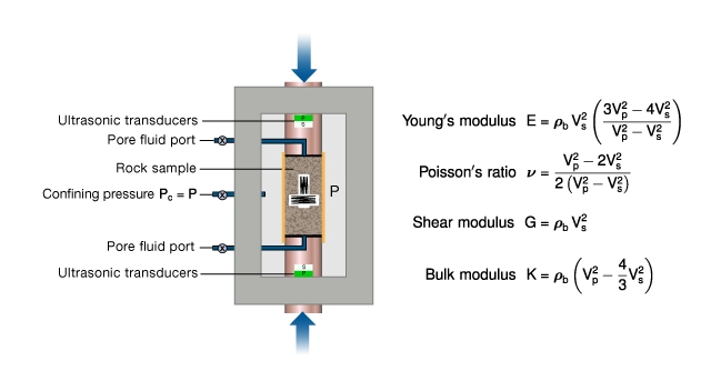
Measuring dynamic moduli for an isotropic rock, Rock mechanical properties, Geomechanics — **Figure 5**: Measuring dynamic moduli for an isotropic rock

Schematic of a triaxial cell fitted with a set of P-wave and S-wave transducers. Simultaneous static and dynamic moduli can be measured in this apparatus.

Transversely Isotropic Rock

The traditional method for measuring the stiffness elements of a TI medium is to invert P and S wave phase velocities that are measured parallel to and perpendicular to the plane of isotropy and measure a “quasi-P-wave” velocity at 45 degrees to the plane of isotropy (Figure 6).

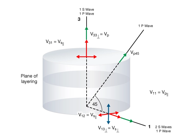
Schematic diagram showing the modes of elastic wave propagation used to determine the five TI moduli, Rock mechanical properties, Geomechanics — **Figure 6**: Schematic diagram showing the modes of elastic wave propagation used to determine the five TI moduli

Given the rock’s bulk density, elastic moduli are calculated using the following relations:

$c_{33}=(\rho \, V_{33})^2$

$c_{11}=(\rho \, V_{11})^2$

$c_{44}=(\rho \, V_{13})^2$

$c_{66}=(\rho \, V_{12})^2$

$c_{13} = -c_{44} + \left [ 4\, \rho^2\, q\, V_{p45}^4 - 2\, \rho \, q\, V_{p45}^{2}\, (c_{11} + c_{33} + 2\, c_{44}) + (c_{11} + c_{44})(c_{33} + c_{44}) \right ]^{\frac{1}{2}}$

In principal, all the measurements can be made on a single sample of rock. This approach minimizes error associated with sample heterogeneity and improves the accuracy of $ c_{13} $. However, measuring all five properties on one core plug requires complex instrumentation inside the pressure vessel. This is possible using technology developed by Jakobsen et al., 2000; Scott and Abousleiman, 2005; Dewhurst and Siggins, 2006.

It is easier and more common to measure the pressure dependence of C in a triaxial cell using the three-plug method. Disadvantages of the three-plug method are the availability of homogeneous samples and the difficulty of obtaining the 45-degree core plugs. (Jones and Wang, 1981; Tosaya, 1982; Hornby, 1998.)

Comparison of Static and Dynamic Moduli

As noted previously, static and dynamic measurements of elastic moduli differ from each other, even on the same volume of rock. This distinction is important because dynamic elastic properties are measured using geophysical methods whereas geomechanics and engineering calculations require static moduli.

In this section we review differences between the static and dynamic Young’s moduli, discuss reasons for the differences between them, and identify when corrections to geophysical data are recommended. The focus is on Young’s modulus because it is a parameter highly correlated to rock strength. It will be shown that much of the difference is attributed to a strain amplitude effect. Confining pressure and fluid saturation also contribute, but to a lesser extent.

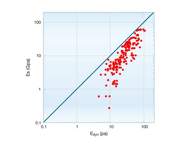
It is commonly observed that the static Young’s modulus, $E_s$ $E_u$ , is systematically lower in magnitude than $E_{dyn}$ . Figure 7 shows a statistical comparison of static, $E_s$ , to dynamic, $E_{dyn}$ , measured on a wide variety of sedimentary rocks. It is clear that $E_{dyn}$ is systematically greater than $E_s$ . Dynamic moduli can be greater than the static moduli by a factor of ten but this difference becomes less in rocks with $E_s \geq$ 20 GPa. The variations shown here are due to the combined effects of lithology, confining pressure, strain amplitude, and fluid saturation.

Static vs dynamic Young's modulus, Rock mechanical properties, Geomechanics — **Figure 7**: Static vs. dynamic Young’s modulus

Simultaneous measurements of static and dynamic moduli provide insight into the possible causes of their differences, which again may be a result of lithology, confining pressure, strain amplitude, and fluid saturation. Figure 8 shows three methods for simultaneous measurement of elastic moduli in a triaxial test. These include:

The static Young’s modulus, $E_s$
$E$ measured using small unload-reload stress cycles, $E_u$
$E_{dyn}$ computed from $V_p$ , $V_s$ and bulk density

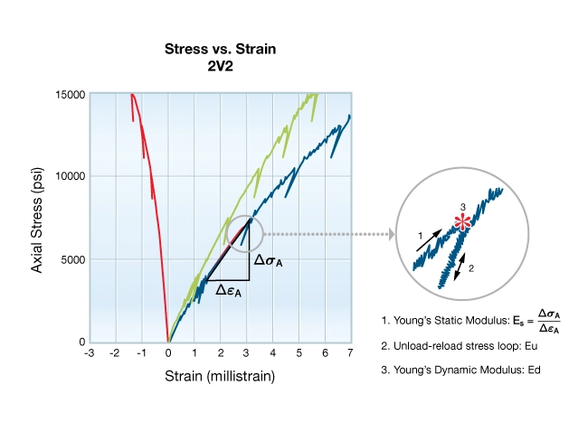
Methods of simultaneous measurements, Rock mechanical properties, Geomechanics — **Figure 8**: Methods of simultaneous measurements

Figure 9 compares simultaneous measurements of Young’s moduli, $E_s$ , $E_u$ and $E_{dyn}$ obtained on a suite of air-dried mudrocks tested by the methods illustrated in Figure 8. Note that the scattering of data is much reduced compared to Figure 7 and that $E_s$ and $E_u$ are both highly correlated with $E_{dyn}$ . Most important is the fact that $E_u$ is much closer to $E_{dyn}$ than it is to $E_s$ . This observation is attributed to the strain amplitude effect reported by Winkler and Nur (1979). Winkler’s experiments showed that elastic modulus became stress sensitive when deformation induced by the testing procedure exceeded strains on the order of 5×10⁻⁷. Beyond this level, the rate of modulus decrease increased as deformation increased. His work suggests that mobilization, an elastic, and plastic processes such as movement along grain boundaries or along faces of microcracks led to reduction of the modulus.

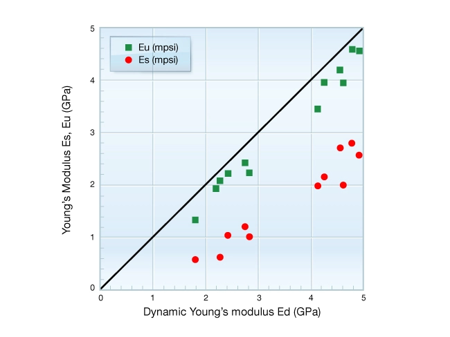
Comparison of simultaneous Young's modulus measurements, Rock mechanical properties, Geomechanics — **Figure 9**: Comparison of simultaneous Young’s modulus measurements

Table 4 shows the magnitude of rock deformation involved in measuring the three different moduli. The greatest modulus corresponds to the least deformation, the lowest modulus to the greatest deformation. For this group of rocks, a ~40% reduction in modulus occurs when sample strains exceed at least 10⁻⁴ and that reduction is probably less.

2\times 10^{-3} — Table 4: Comparison of Rock Deformation Induced Using the Three Methods of Measuring Young’s Modulus

Method	Name	Strain amplitude	Relative magnitude of \( \mathbf{E} \)
Static	$E_{s}$	$2\times 10^{-3}$	$3$
Load-unload	$E_{u}$	$5\times 10^{-4}$	$2$
Dynamic	$E_{dyn}$	$10^{-8}$ $\quad$ to $\quad 10^{-7}$	$1$

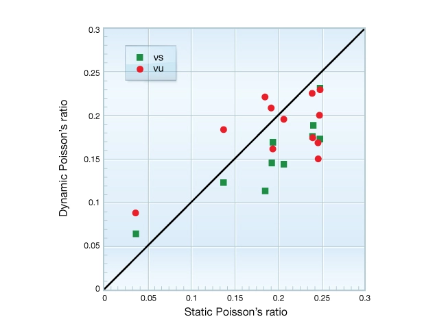
Figure 10 is analogous to Figure 9 and shows how static Poisson’s ratio $\nu_{s}$ compares to $\nu_{u}$ and $\nu_{dyn}$ . In this example, $\nu_{u}$ and $\nu_{dyn}$ are very similar in magnitude but $\nu_{s}$ is systematically lower than $\nu_{dyn}$ . Notice that the scattering of data is greater than for measurements of Young’s modulus however. This tendency is widely observed for measurements of Poisson’s ratio, as it is more difficult to measure experimentally.

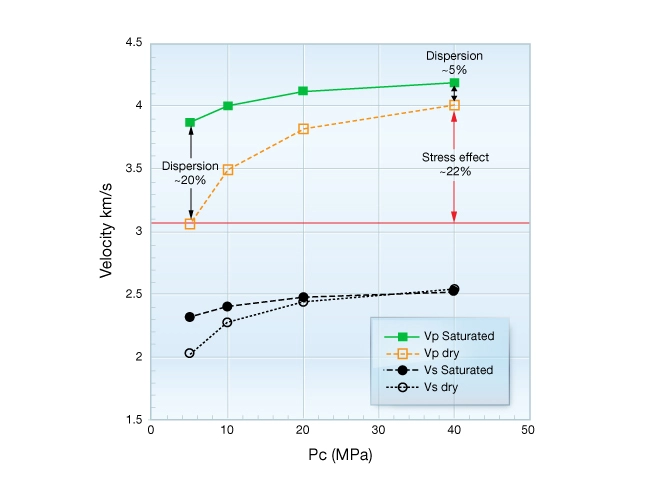
Static Poisson's ratio measurements, Rock mechanical properties, Geomechanics — **Figure 10**: Static Poisson’s ratio measurements

In addition to the dependence of static moduli on strain amplitude, dynamic moduli are affected by fluid saturation. The theory of poroelasticity demonstrates that pore fluids act to stiffen the rock leading to greater elastic wave velocity and greater dynamic moduli. Both the type of fluid (oil, water, gas), and the degree of saturation affect elastic wave velocity, (i.e. dispersion). Figure 11 shows the velocity dispersion measured on dry samples and water saturated samples of Berea sandstone as a function of confining stress. Increases in saturation and effective confining pressure cause velocity increases. Note that fluid saturation affects $V_p$ more than $V_s$ and that the confining stress effects are more pronounced in the dry rock.

Velocity dispersion on dry vs. saturated samples, Rock mechanical properties, Geomechanics — **Figure 11**: Velocity dispersion on dry vs. saturated samples

Rock physics theory cannot account for the systematic variations of elastic moduli measured on rocks. Biot-Gassmann theory may be used to compute dry-frame dynamic moduli from elastic wave velocities, but laboratory experiments are required to correct for strain amplitude and confining pressure effects.

Much of what is currently known about static and dynamic elastic properties pertains to conventional reservoir sandstones and carbonates. Relatively little has been published about unconventional reservoir rocks such as high porosity sand or shale. As a consequence of this and the growing interest in shale gas reservoirs, understanding the difference between $E_s$ and $E _{dyn}$ in anisotropic shale is a current topic of research.