Hydraulic Fracturing Fundamentals

58 minutes read

Fracturing fluids types, Fracture geometry, Frac job design, Hydraulic fracturing techniques, Fracture propagation, Fracking equipment, Fracturing fluid composition, Hydraulic fracturing explained, Fracking techniques, Hydraulic fracturing process, Hydraulic Fracturing, Fracking, Shale Gas Extraction, Fracture Stimulation, Fracturing Fluids, Proppants, Unconventional Oil and Gas, Hydraulic Fracturing Process, Frac Jobs, Fracture Network, Fracture Propagation, Horizontal Drilling, Hydraulic Fracturing Wells, Frac Sand, Well Stimulation, Shale Formation, Fracture Fluids, Fracture Treatment, Fracture Pressure, Reservoir Stimulation, Fracture Design, Fracture Width, Fracture Monitoring, Fracture Optimization, Fracture Mechanics, Hydraulic Fracturing Fundamentals

Qualitative Description of Fracture Growth

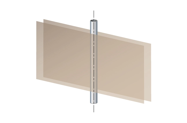
Theoretically, after a fracture is initiated it grows with two opposing wings, each extending into the formation on either side of the wellbore as pumping continues (Figure 1).

Simple model of rectangular two-wing hydraulic fracture with two opposing faces separated by uniform width, Hydraulic Fracturing, Fracturing fluids types, Fracture geometry, Frac job design, Hydraulic fracturing techniques, Fracture propagation, Fracking equipment, Fracturing fluid composition, Hydraulic fracturing explained, Fracking techniques, Hydraulic fracturing process, Hydraulic Fracturing, Fracking, Shale Gas Extraction, Fracture Stimulation, Fracturing Fluids, Proppants, Unconventional Oil and Gas, Hydraulic Fracturing Process, Frac Jobs, Fracture Network, Fracture Propagation, Horizontal Drilling, Hydraulic Fracturing Wells, Frac Sand, Well Stimulation, Shale Formation, Fracture Fluids, Fracture Treatment, Fracture Pressure, Reservoir Stimulation, Fracture Design, Fracture Width, Fracture Monitoring, Fracture Optimization, Fracture Mechanics — **Figure 1**: Simple model of rectangular two-wing hydraulic fracture with two opposing faces separated by uniform width

The increase in fracture volume during a treatment is determined primarily by a material balance with two key elements:

The volume of injected fluid
The portion of injected fluid that leaks off into the formation matrix

The volume of fluid injected is part of the job design. Fluid leakoff is controlled by a number of factors, including the gradual build-up on the fracture face of a thin layer (filter cake) of material carried in the fracturing fluid which results in an ever-increasing resistance to flow through the fracture faces. The ideas behind the leakoff coefficient are that if a filter-cake wall is building up, it will allow less fluid to pass through a unit area in unit time; and the reservoir itself can take less and less fluid if it has been exposed to inflow. Both of these phenomena can be roughly approximated as “square-root time behavior.”

Carter (1957) related the area of a vertical, hydraulically created fracture to the rate of fluid injection and other factors.

$V_L = \dfrac{C_L}{\sqrt{t}}$

Where

$V_L =$ leakoff velocity

$C_L =$ leakoff coefficient

$t=$ time elapsed since start of leakoff process

This equations assumes a uniform fracture width and leakoff flowing perpendicularly across the fracture face at a velocity that is dependent on the duration of flow (Figure 1).

The integrated form of the equation is

$\dfrac{V_{Lost}}{A_L} = C_L\, 2\, \sqrt{t} + S_p$

Where

$V_{Lost} =$ fluid volume passing through fracture surface area from time 0 to time t

$A_L =$ leakoff coefficient fracture surface area

$S_p =$ leakoff coefficient spurt loss coefficient

The fluid volume that passes through the fracture surface during the elapsed time period, divided by the fracture surface area (volume per unit area) is equal to the leakoff coefficient times two times the square root of elapsed time, plus an integration constant. The integration constant is termed the spurt loss coefficient. The two coefficients (leakoff and spurt) can be determined from laboratory tests on core samples.

Fracture Dimensions

For modeling purposes, it is common to model one wing of a hydraulic fracture and assume that the other wing is identical.

For one wing of the fracture at a given time $t$ during treatment at a constant injection rate $q_i$ ,

$V_i = q_i\, t$

Where

$V_i =$ injected volume

$q_i =$ injection rate

$t=$ time elapsed since beginning of treatment

The fluid efficiency $(\eta)$ is the fraction of the injected fluid remaining in the fracture after the rest of the fluid has leaked off into the formation.

$\eta = \dfrac{V}{V_i}$

$V$ is the volume of fluid contained in the fracture, and is equal to the fracture surface area $(A)$ that is, the area of one face of one wing times the average fracture width $(\overline{w})$ .

$V = A\, \overline{w}$

It is often assumed for the purposes of simple models that the created fracture remains within a well-defined lithological layer, and the fracture is therefore characterized by a constant height, $h_f$ .

The fluid injection portion of a single hydraulic fracturing treatment may last from less than an hour to several hours. Points of the fracture face nearest to the well are opened at the beginning of pumping, while the points at the fracture tip are “younger” as the fracture extends into the formation.

Dividing the injected volume by the surface area of one face of one wing results in the so-called “would-be” fracture width. This would-be width consists of the average fracture width, leakoff width and spurt loss width:

$\dfrac{V_i}{A} = \overline{w} + 2\, C_L\, k\, \sqrt{t_e} + 2\, S_p$

The factor 2 is introduced because the fluid leaks off through both faces of one wing.

To obtain an analytical solution for a constant injection rate, Carter (1957) relies on a hypothetical case where the fracture width “jumps” to its final value in the first instant of pumping and the width remains constant during fracture propagation.

Nolte (1986) postulated a similar, but mathematically simpler approach, assuming that the fracture surface evolves according to a power law where the exponent $\textrm{"}\alpha\textrm{"}$ remains constant during the whole injection period.