Hydraulic Fracturing Fundamentals

58 minutes read

Fracturing fluids types, Fracture geometry, Frac job design, Hydraulic fracturing techniques, Fracture propagation, Fracking equipment, Fracturing fluid composition, Hydraulic fracturing explained, Fracking techniques, Hydraulic fracturing process, Hydraulic Fracturing, Fracking, Shale Gas Extraction, Fracture Stimulation, Fracturing Fluids, Proppants, Unconventional Oil and Gas, Hydraulic Fracturing Process, Frac Jobs, Fracture Network, Fracture Propagation, Horizontal Drilling, Hydraulic Fracturing Wells, Frac Sand, Well Stimulation, Shale Formation, Fracture Fluids, Fracture Treatment, Fracture Pressure, Reservoir Stimulation, Fracture Design, Fracture Width, Fracture Monitoring, Fracture Optimization, Fracture Mechanics, Hydraulic Fracturing Fundamentals

Fundamental Concepts of Hydraulic Fracturing

In a hydraulic fracturing treatment, fracturing fluid is injected into the well at treating pressures that are higher than the so-called “formation breakdown pressure.” In practical terms, this pressure corresponds to the minimum horizontal stress that exists within the rock formation. Ideally, this high fluid pressure results in the propagation of a vertically-oriented, two-wing, fracture (Figure 1), which is perpendicular to this minimum horizontal stress.

Idealized depiction of one wing of a vertical hydraulic fracture extending from the wellbore into a formation not to scale, Hydraulic Fracturing, Fracturing fluids types, Fracture geometry, Frac job design, Hydraulic fracturing techniques, Fracture propagation, Fracking equipment, Fracturing fluid composition, Hydraulic fracturing explained, Fracking techniques, Hydraulic fracturing process, Hydraulic Fracturing, Fracking, Shale Gas Extraction, Fracture Stimulation, Fracturing Fluids, Proppants, Unconventional Oil and Gas, Hydraulic Fracturing Process, Frac Jobs, Fracture Network, Fracture Propagation, Horizontal Drilling, Hydraulic Fracturing Wells, Frac Sand, Well Stimulation, Shale Formation, Fracture Fluids, Fracture Treatment, Fracture Pressure, Reservoir Stimulation, Fracture Design, Fracture Width, Fracture Monitoring, Fracture Optimization, Fracture Mechanics — **Figure 1**: Idealized depiction of one wing of a vertical hydraulic fracture extending from the wellbore into a formation (not to scale).

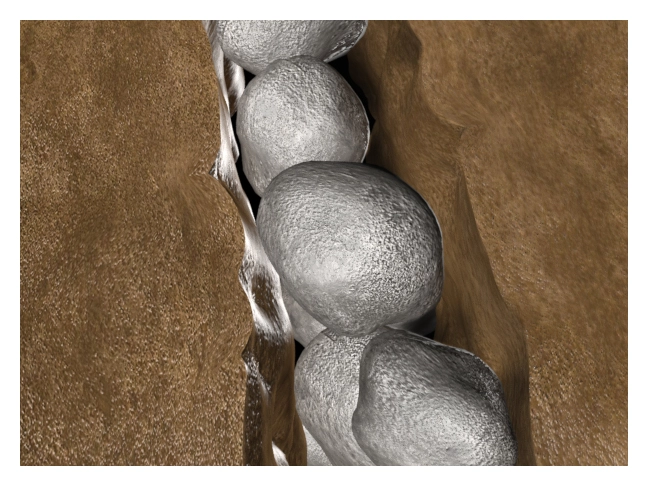
When the created fracture is wide enough to accept them, proppant particles (sand or some other solid material) are mixed with the carrying fluid and injected into the fracture. The proppant material gradually fills up the fracture so that when the pumps are stopped, the proppant keeps the fracture from closing entirely (Figure 2).

Artist's depiction of proppant placed in a fracture before closure, Hydraulic Fracturing, Fracturing fluids types, Fracture geometry, Frac job design, Hydraulic fracturing techniques, Fracture propagation, Fracking equipment, Fracturing fluid composition, Hydraulic fracturing explained, Fracking techniques, Hydraulic fracturing process, Hydraulic Fracturing, Fracking, Shale Gas Extraction, Fracture Stimulation, Fracturing Fluids, Proppants, Unconventional Oil and Gas, Hydraulic Fracturing Process, Frac Jobs, Fracture Network, Fracture Propagation, Horizontal Drilling, Hydraulic Fracturing Wells, Frac Sand, Well Stimulation, Shale Formation, Fracture Fluids, Fracture Treatment, Fracture Pressure, Reservoir Stimulation, Fracture Design, Fracture Width, Fracture Monitoring, Fracture Optimization, Fracture Mechanics — **Figure 2**: Artist’s depiction of proppant placed in a fracture before closure

The propped-open, vertically oriented fracture that results from a successful treatment may be several dozen or several hundred feet high, and extend tens, hundreds, or potentially several thousand feet from the wellbore on either side. Although the fracture is typically just a fraction of an inch wide, it drastically changes the flow characteristics of the formation. Depending on the individual reservoir, this can enhance well productivity by as much as four to six times that of the initial stabilized rate of an un-fractured well.

Basis for Hydraulic Fracturing

Three foundational concepts in hydraulic fracturing relate to:

Near-wellbore damage and skin effects
Productivity index
Dimensionless fracture conductivity and fracture optimization

Near-Wellbore Damage and Skin Effects

Even if the best drilling and completion practices are followed, a certain amount of “damage” or “skin” is created around a wellbore, usually due to one or a combination of:

The infiltration of solid drilling mud particles into the reservoir pore space.
The swelling of formation clays in response to chemical interactions with the drilling fluid.

The resulting skin effect is interpreted as an altered permeability zone an additional, uninvited resistance to hydrocarbon flow.

Figure 3 is a cross-sectional view of a vertical wellbore of radius $r_w$ . Within this radius, there is a region of near-wellbore damage of radius $r_s$ , where “s” indicates skin damage. The permeability of the damaged region ( $k_s$ ) is less than that of the undamaged formation.

Schematic cross-sectional view of a vertical wellbore showing near-wellbore formation damage, Hydraulic Fracturing, Fracturing fluids types, Fracture geometry, Frac job design, Hydraulic fracturing techniques, Fracture propagation, Fracking equipment, Fracturing fluid composition, Hydraulic fracturing explained, Fracking techniques, Hydraulic fracturing process, Hydraulic Fracturing, Fracking, Shale Gas Extraction, Fracture Stimulation, Fracturing Fluids, Proppants, Unconventional Oil and Gas, Hydraulic Fracturing Process, Frac Jobs, Fracture Network, Fracture Propagation, Horizontal Drilling, Hydraulic Fracturing Wells, Frac Sand, Well Stimulation, Shale Formation, Fracture Fluids, Fracture Treatment, Fracture Pressure, Reservoir Stimulation, Fracture Design, Fracture Width, Fracture Monitoring, Fracture Optimization, Fracture Mechanics — **Figure 3**: Schematic cross-sectional view of a vertical wellbore showing near-wellbore formation damage

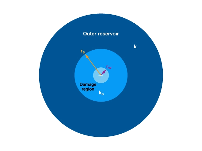
For this simple case of a vertical well, where flowing fluid is converging radially toward the wellbore, this reduced permeability results in a large pressure drop and a subsequent decrease in well productivity. In this instance, the objective of a hydraulic fracture treatment is to create a fracture that extends beyond the damaged region, bypassing the zone of reduced permeability and thereby improving the well’s productivity.

Productivity Index

The objective of any fracture stimulation treatment in a producing well is to increase the productivity index (J):

$J = \dfrac{q}{\overline{P}_R - P _{wf}}$

Where

$q$ = flow rate,

$\overline{P}_R - P _{wf} =$ pressure drawdown, which is equal to the difference between the average reservoir pressure ( $\overline{P}_R$ ) and the flowing bottomhole pressure ( $P _{wf}$ ).

The productivity index can b increased in either of two ways:

Increase the production rate for a given pressure drawdown this has historically been the goal of hydraulic fracture stimulations.
Decrease the pressure drawdown for a specified production rate this is the basis for using hydraulic fracturing to solve sand control or other drawdown-sensitive production problems.

Productivity Index and Skin Factor

For a well producing under pseudosteady-state flow conditions in a bounded circular reservoir, the productivity index is approximated as:

$J \approx \dfrac{2\, \pi \, k\, h}{B\, \mu} \cdot \dfrac{1}{-0.75 + \ln \left( \frac{r_e}{r_w} \right)+ s}$

Where

$k$ = permeability

$h$ = formation thickness

$B$ = formation volume factor

$μ$ = fluid viscosity

$r_e$ = well’s drainage area radius

$r_w$ = wellbore radius

$s$ = skin factor

For radial flow in gas wells, a similar relationship applies:

$\Delta P = \dfrac{\overline{P}_R^2 - P _{wf}^2}{P _{sc}}$

$J \approx \dfrac{2\, \pi \, k\, h\, T_{sc}}{\mu\, ZT} \cdot \dfrac{1}{-0.75 + \ln \left( \frac{r_e}{r_w} \right)+ s}$

where μ is the average gas viscosity, Z is the average compressibility factor, T is the temperature and the subscript sc refers to standard conditions.

When all other parameters are constant, an oil or gas well’s flow rate decreases as the skin factor increases.

The Hawkins formula can be used to express the skin factor in terms of the permeability in the damaged zone and the radius of the damaged zone (Figure 3):

$s = \left( \dfrac{k}{k_s} - 1 \right)\, \ln \dfrac{r_s}{r_w}$

This formula indicates that:

For an undamaged well (ks=k), s=0
For a damaged well (k_s<k), s>0
If the permeability impairment is several-fold, a relatively small damage radius is enough to cause a significant positive skin effect. In other words, radial flow is very sensitive to near-well damage.

Well Stimulation to Improve Productivity Index

Well stimulation was originally introduced as a way to reduce the skin effect to zero by “restoring” the permeability in the damaged zone to the original formation permeability. Sandstone matrix acidizing, where the idea is to dissolve drilling mud solids or other particles that cause near-well damage, is one such type of stimulation. This type of matrix treatment does not change the original flow paths of the formation fluids.

In carbonate reservoirs, matrix acidizing may actually dissolve part of the rock matrix in addition to removing formation damage. This creates a near-wellbore zone of enhanced permeability, where k/k_s<1. The skin factor in this case is negative, indicating that the post-treatment flow conditions are better than existed in the original undamaged formation. It is not even necessary to eliminate all of the damage; it is enough that the treatment creates enough flow capacity near the well to bypass the damaged zone.

The idea of a hydraulic fracturing treatment is to create a conductive fracture by driving a “fluid wedge” through the rock. A solid propping agent is then placed in the fracture to prevent it from closing.

(An alternative to the propped fracture is a process called acid fracturing, which uses a low-pH fluid to dissolve a portion of the rock on the fracture face. This leaves the two etched surfaces unable to close on each other, and therefore a high-conductivity conduit remains in the formation.)

Propped fracturing serves to not only bypass the damaged zone, but by superimposing a highly conductive planar conduit on the formation, it changes the geometric structure of the flow paths or “streamlines,” thereby significantly increasing the productivity index.

One way to numerically characterize the effect of a propped fracture is to introduce the pseudo-skin factor, s_f. (Cinco-Ley and Samaniego, 1979).

$J_f \approx \dfrac{2\, \pi \, k\, h}{B\, \mu} \left [\dfrac{1}{-0.75 + \ln \left( \frac{r_e}{r_w} \right)+ s_f} \right ]$

Where

J_f= post-treatment productivity index

k= formation permeability

h= formation thickness

B= formation volume factor

μ= viscosity

r_e= well drainage radius

r_w= wellbore radius

s_f= pseudo skin factor

A propped fracture that bypasses formation damage results in a negative pseudo-skin factor. The question is how to predict the pseudo-skin factor that will result from a given treatment, knowing the relevant formation and fracture properties. Being able to answer this question is the key to optimizing the treatment.

Dimensionless Fracture Conductivity and Fracture Optimization

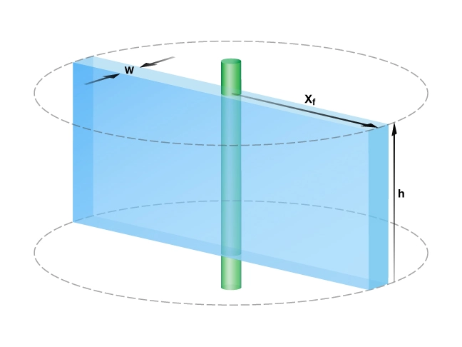
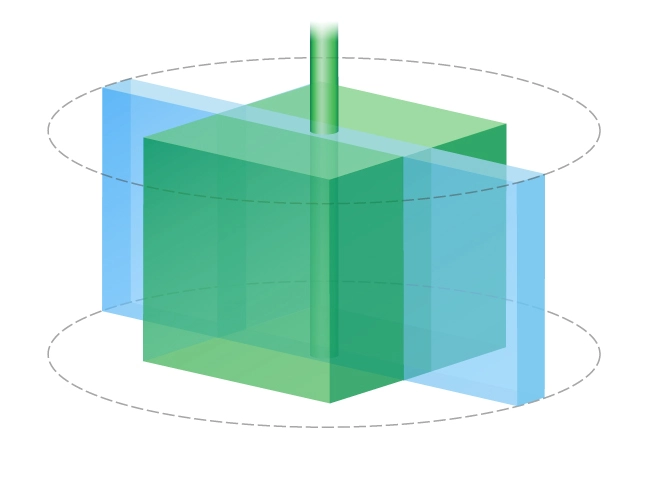
In keeping with Cinco-Ley’s and Samaniego’s concept of a pseudo-skin factor, assume a fully penetrating rectangular fracture, in which the fracture height and formation thickness are equal (Figure 4). The fracture half-length x_f is the length of one wing of a fracture. Assume that two symmetrical fracture wings are created simultaneously during a fracture operation, with the total overall length equal to twice the half-length.

Idealized, fully penetrating rectangular fracture with a height (h) equal to the formation thickness and a fracture half-length (xf) equal to one wing of the fracture, Hydraulic Fracturing, Fracturing fluids types, Fracture geometry, Frac job design, Hydraulic fracturing techniques, Fracture propagation, Fracking equipment, Fracturing fluid composition, Hydraulic fracturing explained, Fracking techniques, Hydraulic fracturing process, Hydraulic Fracturing, Fracking, Shale Gas Extraction, Fracture Stimulation, Fracturing Fluids, Proppants, Unconventional Oil and Gas, Hydraulic Fracturing Process, Frac Jobs, Fracture Network, Fracture Propagation, Horizontal Drilling, Hydraulic Fracturing Wells, Frac Sand, Well Stimulation, Shale Formation, Fracture Fluids, Fracture Treatment, Fracture Pressure, Reservoir Stimulation, Fracture Design, Fracture Width, Fracture Monitoring, Fracture Optimization, Fracture Mechanics — **Figure 4**: Idealized, fully penetrating rectangular fracture with a height (h) equal to the formation thickness and a fracture half-length (*x_f*) equal to one wing of the fracture

The starting point in determining the optimal fracture dimensions is the radial flow equation for the post-hydraulic fracturing productivity index:

$J_f \approx \dfrac{2\, \pi \, k\, h}{B\, \mu} \left [\dfrac{1}{-0.75 + \ln \left( \frac{r_e}{r_w} \right)+ s} \right ]$

This equation is expanded to show the direct relationship between the fracture half-length and the productivity index.

$J_f \approx \dfrac{2\, \pi \, k\, h}{B\, \mu} \cdot \dfrac{1}{-0.75 + \ln \frac{r_e}{x_f} + \left (s + \ln\frac{x_f}{r_w} \right ) }$

The dimensionless factor f, which does not refer to a wellbore radius, is then substituted in place of the pseudo-skin factor.

$J_f \approx \dfrac{2\, \pi \, k\, h}{B\, \mu} \cdot \dfrac{1}{-0.75 + \ln \left( \frac{r_e}{x_f} \right) + f }$

While the two forms of the productivity index are algebraically equivalent, the expanded form is physically more meaningful. The expanded form of the denominator involves three terms:

The first term, -0.75, is present because the pressure drawdown is defined in terms of average pressure.
The second term, $\ln \left( \dfrac{r_e}{x_f} \right)$ , represents the effect of the fracture half-length.
The third term, $f$ , represents the effect of a combination of fracture variables called dimensionless fracture conductivity, $C _{fD}$ ,

$C _{fD} \approx \dfrac{k_f \overline{w}}{k\, x_f}$

Where

$k$ = the reservoir permeability

$x_f$ = the half-length of the propped fracture

$k_f$ = the permeability of the proppant pack within the fracture

$\overline{w}$ = the average fracture width

The dimensionless fracture conductivity defined here should not be confused with the dimensioned fracture conductivity, which is equal to kf w. The dimensionless fracture conductivity expresses how the two primary functions of the fracture are related. These two functions are:

To collect the hydrocarbon fluids from the surrounding matrix rock, and
To conduct the hydrocarbon fluids collected inside the fracture to the wellbore.

If $C_{fD}$ ≪1, flow within the fracture is restricted, but flow into the fracture from the surrounding matrix is relatively unrestricted.

If $C_{fD}$ ≫1, flow within the fracture is unrestricted, but flow from the surrounding matrix into the fracture is relatively restricted.

The expanded form of the post-treatment productivity index indicates that post-treatment performance is not related to the wellbore radius and the original skin factor. This is how it should be, because the radial streamline structure has been changed and the fracture bypasses the pre-treatment damage.

The key to understanding hydraulic fracturing is that the dimensionless factor, $f$ , depends on $C_{fD}$ only. The most well-known graphical representation of the function $f(C_{fD})$ was given by Cinco-Ley and Samaniego, (1981) as shown in Figure 5.

Dimensionless factor, f, as a function of CfD, Hydraulic Fracturing, Fracturing fluids types, Fracture geometry, Frac job design, Hydraulic fracturing techniques, Fracture propagation, Fracking equipment, Fracturing fluid composition, Hydraulic fracturing explained, Fracking techniques, Hydraulic fracturing process, Hydraulic Fracturing, Fracking, Shale Gas Extraction, Fracture Stimulation, Fracturing Fluids, Proppants, Unconventional Oil and Gas, Hydraulic Fracturing Process, Frac Jobs, Fracture Network, Fracture Propagation, Horizontal Drilling, Hydraulic Fracturing Wells, Frac Sand, Well Stimulation, Shale Formation, Fracture Fluids, Fracture Treatment, Fracture Pressure, Reservoir Stimulation, Fracture Design, Fracture Width, Fracture Monitoring, Fracture Optimization, Fracture Mechanics — **Figure 5**: Dimensionless factor, $<em>f$ , as a function of *$C_{fD}$* with best fit equation for purple line

**Figure 5**: Dimensionless factor, $<em>f$ , as a function of *$C_{fD}$* with best fit equation for purple line

When the dimensionless fracture conductivity is high ( $C_{fD} > 100$ , which is possible for low permeability formations having undergone a massive hydraulic fracturing treatment), the behavior is similar to that of an infinite conductivity fracture (Gringarten and Ramey, 1974).

For an infinite conductivity fracture, the dimensionless factor f is equal to $\ln 2$ , indicating that the fractured well produces similarly to a hypothetical well of enlarged radius equal to $x_f/2$ . Such an infinite conductivity behavior is, however, impossible to achieve in most formations except for those with very low permeability. In medium and high permeability formations, the propped fracture is always of finite conductivity.

In a finite conductivity fracture, there are two physical factors (fracture length and fracture width) competing for the same resource: an incremental amount of propping agent. The propping agent serves to increase fracture length or fracture width.

Before the advent of tip screenout (TSO) techniques, fracture length and width were difficult to influence separately. The TSO technique introduced a significant change to design philosophy by making it possible to increase fracture width without increasing the fracture extent. This makes it possible to optimize both fracture length and width for a given proppant volume.

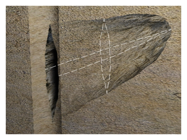
The solution to this optimization problem is of primary importance in understanding hydraulic fracturing (Prats, 1961). The same propped volume can be used to create a narrow, elongated fracture or a wide, short fracture (Figure 6).

Schematic showing two alternative solutions for the same proppant volume, Hydraulic Fracturing, Fracturing fluids types, Fracture geometry, Frac job design, Hydraulic fracturing techniques, Fracture propagation, Fracking equipment, Fracturing fluid composition, Hydraulic fracturing explained, Fracking techniques, Hydraulic fracturing process, Hydraulic Fracturing, Fracking, Shale Gas Extraction, Fracture Stimulation, Fracturing Fluids, Proppants, Unconventional Oil and Gas, Hydraulic Fracturing Process, Frac Jobs, Fracture Network, Fracture Propagation, Horizontal Drilling, Hydraulic Fracturing Wells, Frac Sand, Well Stimulation, Shale Formation, Fracture Fluids, Fracture Treatment, Fracture Pressure, Reservoir Stimulation, Fracture Design, Fracture Width, Fracture Monitoring, Fracture Optimization, Fracture Mechanics — **Figure 6**: Schematic showing two alternative solutions for the same proppant volume

It is convenient to select $C_{fD}$ as the decision variable, and then to express the fracture half-length using the propped volume of one wing $V_f$ .

$x_f = \left( \dfrac{V_f\, k_f}{C_{fD}\, h\, k } \right)^{\frac{1}{2}}$

Substituting this equation into the radial flow equation,

$J \approx \dfrac{2\, \pi \, k\, h}{B\, \mu} \cdot \dfrac{1}{-0.75 + 0.5\ln\left (\frac{r_e^2\, h\, k}{V_f \, k_f} \right ) + 0.5\ln C_{fD} + f \left (C_{fD} \right )}$

results in a relationship in which the only unknown is $C_{fD}$ :

$y = 0.5\ln C_{fD} + f \left (C_{fD} \right )$

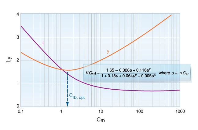
Since the drainage radius, formation thickness, formation and fracture permeabilities and the propped volume are fixed, the maximum productivity index occurs when the quantity $y$ reaches its minimum (Figure 7). This minimum value of $y$ depends only on $C_{fD}$ , and occurs when $C_{fD}$ is equal to 1.6. This is true for any reservoir and any fixed amount of proppant.

Quantity y as a function of CfD showing minimum at a value of 1.6, the optimum value for dimensionless fracture conductivity, Hydraulic Fracturing, Fracturing fluids types, Fracture geometry, Frac job design, Hydraulic fracturing techniques, Fracture propagation, Fracking equipment, Fracturing fluid composition, Hydraulic fracturing explained, Fracking techniques, Hydraulic fracturing process, Hydraulic Fracturing, Fracking, Shale Gas Extraction, Fracture Stimulation, Fracturing Fluids, Proppants, Unconventional Oil and Gas, Hydraulic Fracturing Process, Frac Jobs, Fracture Network, Fracture Propagation, Horizontal Drilling, Hydraulic Fracturing Wells, Frac Sand, Well Stimulation, Shale Formation, Fracture Fluids, Fracture Treatment, Fracture Pressure, Reservoir Stimulation, Fracture Design, Fracture Width, Fracture Monitoring, Fracture Optimization, Fracture Mechanics — **Figure 7**: Quantity *$y$* as a function of *$C_{fD}$* 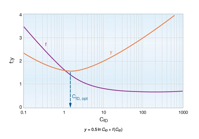showing minimum at a value of 1.6, the optimum value for dimensionless fracture conductivity

Fracture Optimization

The optimal dimensionless fracture conductivity corresponds to the best compromise between the fracture’s capacity to conduct hydrocarbons and the reservoir’s capacity to deliver hydrocarbons subject to the constraint that the fracture volume is fixed at some prescribed value.

Fracture Length and Width

Once the volume of proppant that can be placed into one wing of the fracture $(V_f)$ is known, we can calculate the optimal fracture dimensions $x_f$ and w by substituting the value of 1.6 for $C_{fD}$ in the equations for fracture half-length and fracture width:

$x_f = \left( \dfrac{V_f\, k_f}{1.6\, h\, k } \right)^{\frac{1}{2}}$

$w = \left( \dfrac{1.6V_f\, k}{h\, k_f } \right)^{\frac{1}{2}}$

We can also solve for $y$ at the optimum dimensionless fracture conductivity and substitute into the productivity index equation to express the productivity index for a hydraulically fractured well with an optimal compromise between fracture width and length for a given fracture volume.

$y _{opt} = 0.5\ln (1.6) + f(1.6) = 1.619$

$y _{opt} - 0.75 = 0.869$

$J _{f,\, opt} = \dfrac{2\, \pi \, k\, h}{B\, \mu} \cdot \dfrac{1}{0.869 + 0.5\ln \left( \frac{r_e^2\, h\, k}{V_f\, k_f} \right)}$

This relationship reveals a number of insights into the nature of hydraulically induced fractures:

There is no theoretical difference between low and high permeability formation fracturing. In both cases, there exists a technically optimum fracture, and in both cases it should have a dimensionless fracture conductivity of 1.6.
- In a low matrix permeability formation, this requirement results in a long and narrow fracture.
- In a high matrix permeability formation, a short and wide fracture will provide the same optimal dimensionless conductivity.
Increasing either the proppant volume or the permeability of the proppant pack by a given factor (for example, 2) has exactly the same effect on productivity, so long as the proppant is optimally placed.
The skin improvement depends on the amount of proppant (or on the proppant pack permeability) according to a log-square-root relation.
To achieve the same post-treatment skin factor in a low and a high permeability formation, the volume of proppant should be increased by the same factor as the ratio of the formation permeability, provided all the other formation and proppant parameters are the same.

The above relationships shed light on the role of the individual variables and provide for the theoretically optimum placement of a given amount of proppant. In practice, however, there may be a number of factors that force a departure from this theoretical optimum:

Since not all proppant will be placed into the productive (permeable) layer, the optimum length and width should be calculated using the effective proppant volume, subtracting the proppant placed into the non-productive layers.
In very low permeability formations, the indicated fracture width might be too small (where the permeability of the proppant pack cannot be considered constant), so a minimum width limit should be applied.
In very high permeability formations, the indicated fracture length might not be enough to bypass a large damaged zone, therefore a minimum length should be applied.
Considerable fracture width can be lost because of proppant embedment into soft formations when the fracture closes after fracturing pressure is released.
For gas wells, non-Darcy flow effects may create a dependence of the apparent permeability of the proppant pack on the production rate itself.
Strictly speaking, the Cinco-Ley and Samaniego pseudo skin factor is valid only for $x_f \ll 1$ and at later flow times. Fortunately, for moderate and high permeability formations $(k \gg 1\, md)$ , the above conditions are likely to be fulfilled.

Transient flow regimes, deep penetration of the fracture relative to the drainage area, and other phenomena may also modify the optimal compromise between width and length, but these issues are of secondary importance.

The pseudo-skin factor concept is not the only possible option for visualizing the effect of a fracture treatment. We could also derive all of the above results using the concept of equivalent wellbore radius. We have to be very cautious not to use both the pseudo-skin factor and the equivalent wellbore radius at the same time, however, because that might lead to accounting for the same effect twice.

Proppant Volume

Having settled the optimization of fracture length vs. width for a fixed proppant volume, the remaining task is to determine what proppant volume is optimal for a given treatment.

From a technical standpoint, the more proppant that is placed in the formation, the better the well’s post-treatment performance will be. But at some point, economic considerations take over. The additional revenue from a larger propped volume eventually becomes marginal compared to the more-than-linearly increasing costs. This situation is best addressed using a Net Present Value (NPV) analysis, based on predictions of well performance under varying proppant volumes.

Once the optimum dimensionless fracture conductivity is understood, fracture length and width are no longer freely selectable design parameters. From the production engineer’s point of view, the amount of proppant (propped volume) should be the primary variable characterizing the treatment size.