Rock Mechanical Properties

Geophysical Methods for Measuring Elastic Properties

Sonic logging is the most common method of measuring rock elastic moduli at depth in sedimentary basins. Inversion of geophysical measurements of bulk density and compressional and shear wave velocities yield dynamic elastic moduli. Measurements made with wireline or logging while drilling tools provide the most accurate data with highest vertical resolution. The elastic parameters of isotropic rocks may be calculated from standard sonic and seismic data. However, only a partial set of the TI parameters can be obtained from standard logging or seismic methods.

Elastic Properties from Borehole Methods

Sonic logging provides the only continuous-direct measurement of rock elastic properties at any significant depth in sedimentary basins. Initially, sonic tools were only deployed on a wireline. Then monopole sonic logging while drilling (LWD) measurements became available. Features that all sonic logging tools have in common are:

• Sources that excite elastic waves in the rock and borehole fluids
• Receivers that detect the arrival of elastic waves
• Downhole processors that digitally record the received waveforms

Recorded waveforms are processed to determine the slowness (transit time) of compressional waves, , shear waves, , and Stoneley waves, . Slowness is simply the inverse of velocity such that, , and . The dynamic elastic moduli for isotropic rocks can be computed from , , plus bulk density, .

Young’s modulus
Poisson’s ratio
Shear modulus
Bulk modulus

Monopole Tools

Monopole tools have a single acoustic source, usually located below an array of receivers (Aron et al., 1978). The source and receivers are separated by an attenuating section to suppress signals propagating along the tool from reaching the receivers first. Compressional, shear, and Stoneley wave slownesses are obtained by processing waveforms recorded by the tool. Slownesses are normally expressed in units of microseconds per foot (s/ft).

Monopole tools have a practical limitation in that they do not provide data when the formation slowness is less than the slowness of the drilling mud (that is, is greater than about 180 (s/ft). When this occurs, elastic waves are refracted away from the borehole and do not reach the receiver array.

Figure 1 shows a schematic of a digital sonic tool and the waveforms recorded by the receiver array.

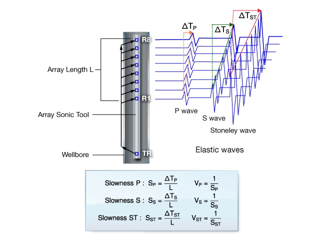
Shown are the acoustic transmitter (TR) an array of receivers (R1…R8), and idealized waveforms recorded by the receiver array for each firing of the transmitter. Compressional, shear, and Stoneley wave slownesses are computed by detecting their move outs across the array. The slownesses are referenced to the depth corresponding to the center of the receiver array. When the sonic log is run in combination with a density log, the two data sets can be merged, depth shifted, and processed to produce a continuous log of dynamic elastic parameters: , , , . Note that in fluid saturated rocks, these moduli represent undrained moduli. In gas saturated rocks they represent the dry-frame moduli. Corrections are required to determine static-drained moduli, as discussed in the previous section.

Dipole Tools

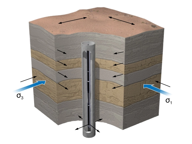
Cross-dipole logging tools were developed to overcome limitations of the monopole tools in slow high-porosity formations where refracted waves are not recorded. These tools contain two dipole transmitters and two receiver arrays. Figure 2 shows the schematic of a dipole sonic tool in a vertical borehole drilled perpendicular to bedding showing orthogonal transmitters and receivers. Notice that the fast shear wave may propagate parallel to the maximum horizontal stress, natural fractures, or both.

Each receiver array is coplanar with one transmitter. The two coplanar-transmitter-receiver pairs are positioned orthogonal to each other. Each dipole transmitter excites a dispersive flexural borehole mode that is polarized in the plane of the dipole source. The low frequency limit of the dispersive flexural mode propagates at the formation shear velocity.

Dipole logging tools typically contain a monopole source in addition to two dipole sources. The monopole source excites compressional and Stoneley waves while the dipole transmitters excite flexural waves. Computer processing extracts the shear velocity from waveforms recorded by each receiver array. Compressional and Stoneley-wave velocities are determined in the same manner as the monopole tools.

The dipole tools can record shear slownesses as low as 450 s/ft and more. However, when the formation compressional slowness is greater than fluid slowness, compressional waves are not detectable. In these situations, only a shear modulus can be measured.

Elastic anisotropy can be detected and partly quantified using dipole sonic tools. If the formation is isotropic or isotropic in the plane perpendicular to the wellbore (such as a TI-V formation), the two shear slownesses are the same. If the formation, in the plane perpendicular to the borehole, is anisotropic, shear wave splitting occurs and the flexural modes will propagate at different velocities in orthogonal planes, aligned with an axis of elastic symmetry (Plona et al., 2000). Processing of dipole sonic data yields a fast and slow shear velocity, or simply a fast shear and a slow shear. When the dipole tool is combined with an orientation device, the azimuth of the fast and slow shear waves can be determined. We will expand on this subject later when discussing borehole stresses.

Waveforms recorded by sonic tools which have both monopole and dipole sources can be processed to yield up to four of the five elastic stiffness parameters that characterize a TI material. Four stiffness parameters can be measured when the borehole is perpendicular to sedimentary layering, . and are obtained from the velocity of shear waves propagating perpendicular to layers and polarized in the plane of the layers and . is obtained from the velocity of shear waves propagating and polarized in the plane of layering . This velocity is not measured directly but is modeled from the Stoneley wave slowness.

For a borehole drilled perpendicular to bedding in a TI material, equals so only three independent parameters are measured directly. Missing for the TI medium are and .

In some cases the missing stiffnesses can be estimated using the ANNIE approximation (Shoenberg et al., 1996).

Formations that have elastic symmetry lower than TI may be detected but not fully characterized. For example, it is not unusual for a vertical well to encounter naturally-fractured horizontally-bedded shale. If only one set of vertical fractures are present, will not equal . This formation would be characterized by orthorhombic elastic symmetry requiring nine independent stiffness parameters.

Quantifying the stiffness parameters gets complicated quickly whenever the borehole is inclined to a plane of elastic symmetry. Special software is required to process and interpret such data and laboratory measurements on core are required to quantify all the moduli. A prudent approach to working with rock anisotropy is to focus on sections of the log where the borehole is aligned normal to the plane of isotropy or a plane of elastic symmetry (Sinha et. al, 2006).

Elastic Properties from Surface Seismic

Surface seismic may be processed to reveal spatial trends in rock mechanical properties. Inversion of amplitude versus offset (AVO) data yields 3D volumes, or “cubes” of P-wave impedance, , the ratio , and bulk density, . In theory this is all the information required to calculate cubes of elastic moduli for an isotropic material. However, the density cube is the least accurate of the inversion products. If the density cube can be calibrated, and cubes and isotropic elastic moduli cubes can be generated. A 3D estimate of the elastic moduli enables one to compute 3D estimates of rock strength and earth stresses.

Anisotropy is revealed in seismic data when and are found to be path dependent. In anisotropic formations, and are typically faster for waves propagating parallel to sedimentary layering than perpendicular to it. This observation reinforces the idea that large-scale sedimentary sequences are characterized by TI-V elastic symmetry. In cases where natural fracturing causes the velocity anisotropy, a TI-H model often fits the data. Although the existence and relative strength of TI anisotropy can be determined from seismic data, the numerical values of the stiffness parameters are not rigorously quantified.

Keep in mind that seismic waves respond to average elastic properties over a distance equal to the wavelength, about 25 m (+/-). Thus comparison to sonic may or may not be straight forward. Nevertheless, the low spatial-frequency depth trends of the two data sets should be similar. And large scale spatial variations in rock mechanical properties, derived from 3D seismic data, are useful for exploration and field development planning.