Mechanical Earth Model | What is a mechanical earth model?

23 minutes read

The Mechanical Earth Model, Geomechanics, Geomechanical model, geomechanical properties, Building geomechanical models

Step 5: Rock Strength

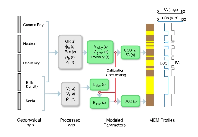
Profiles of the rock strength parameters are derived from data used to construct the mechanical stratigraphy and elastic property profiles. The unconfined compressive strength (UCS) can be estimated from lithology and porosity data or from the static Young’s modulus. If the lithology-porosity approach is used, separate models for grain-support and clay-support facies apply. Friction angle (FA) is computed from $ V_{grain} $ obtained from the volumetric analysis defining the mechanical stratigraphy in Step 4.

Unconfined compressive strength and friction angle are calibrated to laboratory triaxial strength measurements made on cores. Calibration is recommended whenever possible but particularly when using the lithology-porosity model, UCS variations within a single reservoir section, carbonate lithologies, and any rock with porosity >25%.

Figure 6 illustrates methods for constructing profiles of rock strength parameters: unconfined compressive strength (UCS) and friction angle (FA). Calibration points are shown by red lines.

Rock Strength, The Mechanical Earth Model MEM,Mechanical Earth Model,Geomechanics,Rock properties,Stress distribution,Strain,Elastic deformation,Plastic deformation,Shear strength,Fracture mechanics,Faults,Pore pressure,Rock mechanics,Reservoir simulation,Wellbore stability,Rock failure,Rock strength,Geotechnical analysis,Formation evaluation,Borehole stability,Rock behavior,Stress-strain relationship,Deformation analysis,Rock physics,Geostress,Mechanical properties,Mechanical Earth Model,Geomechanics,Geomechanical Analysis,Earth Model,Understanding Earth's Mechanics,Advanced Geomechanics,Mechanical Earth Model,Geomechanics,Earth Model,Geomechanical Analysis,Understanding Earth's Mechanics,Advanced Geomechanics,Earth Modeling Techniques,Geomechanical Properties,Mechanical Behavior of Earth,Geomechanical Modeling,Earth Stress Analysis,Introduction to Geomechanics,Earth Deformation Analysis,Geomechanical Engineers,Earth Material Properties,Geomechanical Testing,Earth Stress Modeling,Application of Geomechanics,Geomechanical Consultants,Earth Stability Analysis,Geomechanical Software,Earth Mechanics Principles — **Figure 6**: Inputs for determining rock strength

Earth Stresses

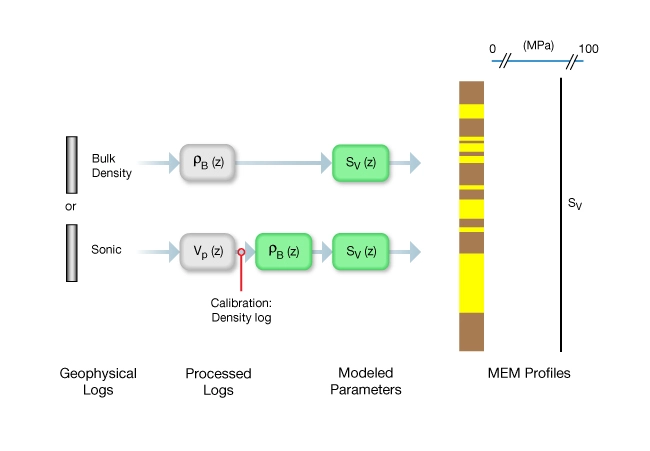
Step 6: Overburden Stress

Overburden stress is calculated by integrating bulk density over depth (Figure 7). This requires a density log run to the surface or a formation density estimate between the top of the logged interval and the surface. Exploration wells typically run density and sonic logs to surface. If density logs to surface are not available, a density profile is constructed using density and or sonic logs from offset wells over the stratigraphic section of interest. Gardner’s method is commonly used to model the density profile from compressional wave velocity.

$\rho_b = \alpha V^\beta _p$

In general, there is no direct calibration for the vertical stress. Occasionally hydraulic fracturing stress measurements measure the vertical stress but this is the exception when the induced fractures propagate in a horizontal plane. The primary opportunity to improve the overburden stress model is to measure bulk density over sections where it had been modeled.

Figure 7 illustrates methods for constructing a profile of the overburden or vertical stress $S_V$ .

Overburden Stress, The Mechanical Earth Model MEM,Mechanical Earth Model,Geomechanics,Rock properties,Stress distribution,Strain,Elastic deformation,Plastic deformation,Shear strength,Fracture mechanics,Faults,Pore pressure,Rock mechanics,Reservoir simulation,Wellbore stability,Rock failure,Rock strength,Geotechnical analysis,Formation evaluation,Borehole stability,Rock behavior,Stress-strain relationship,Deformation analysis,Rock physics,Geostress,Mechanical properties,Mechanical Earth Model,Geomechanics,Geomechanical Analysis,Earth Model,Understanding Earth's Mechanics,Advanced Geomechanics,Mechanical Earth Model,Geomechanics,Earth Model,Geomechanical Analysis,Understanding Earth's Mechanics,Advanced Geomechanics,Earth Modeling Techniques,Geomechanical Properties,Mechanical Behavior of Earth,Geomechanical Modeling,Earth Stress Analysis,Introduction to Geomechanics,Earth Deformation Analysis,Geomechanical Engineers,Earth Material Properties,Geomechanical Testing,Earth Stress Modeling,Application of Geomechanics,Geomechanical Consultants,Earth Stability Analysis,Geomechanical Software,Earth Mechanics Principles — **Figure 7**: Inputs for determining overburden stress

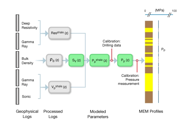
Step 7: Pore Pressure

The pore pressure ( $P_p$ ) profile is modeled through shale sections using Bowers’ or Eaton’s methods. Both methods can take compressional wave velocity ( $V_p$ ), and deep resistivity and overburden stress $S_V$ as input data. Pressure in adjacent permeable formations is assumed to be in equilibrium with the shale except when the centroid effect must be taken into account. Figure 8 shows this process schematically. The pressure in the shales (clay-supported rocks colored brown) is depicted with a solid line. The inferred pressure in the permeable beds (grain-supported facies, colored yellow) is represented by a dotted line.

It is very important to calibrate the pore pressure profile because of its impact on drilling safety and earth stress calculations. Uncalibrated pore pressure profiles often show general trends of pressure vs. depth but the magnitude of pressure can be seriously in error. Mud weights used to drill the well and reports of losses or influxes of formation fluid (called kicks) are used for calibration. The best calibration is obtained from direct measurement of formation pressure or by well testing in reservoir sections.

Pore pressure, The Mechanical Earth Model MEMmMechanical Earth Model,Geomechanics,Rock properties,Stress distribution,Strain,Elastic deformation,Plastic deformation,Shear strength,Fracture mechanics,Faults,Pore pressure,Rock mechanics,Reservoir simulation,Wellbore stability,Rock failure,Rock strength,Geotechnical analysis,Formation evaluation,Borehole stability,Rock behavior,Stress-strain relationship,Deformation analysis,Rock physics,Geostress,Mechanical properties,Mechanical Earth Model,Geomechanics,Geomechanical Analysis,Earth Model,Understanding Earth's Mechanics,Advanced Geomechanics,Mechanical Earth Model,Geomechanics,Earth Model,Geomechanical Analysis,Understanding Earth's Mechanics,Advanced Geomechanics,Earth Modeling Techniques,Geomechanical Properties,Mechanical Behavior of Earth,Geomechanical Modeling,Earth Stress Analysis,Introduction to Geomechanics,Earth Deformation Analysis,Geomechanical Engineers,Earth Material Properties,Geomechanical Testing,Earth Stress Modeling,Application of Geomechanics,Geomechanical Consultants,Earth Stability Analysis,Geomechanical Software,Earth Mechanics Principles — **Figure 8**: Inputs for determining pore pressure

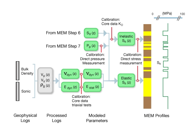
Step 8: Least Horizontal Stress Model

A lithology-dependent profile of the least horizontal stress can be constructed using one of the following models:

Uniaxial consolidation model (inelastic model) requiring a mechanical stratigraphy, overburden stress, pore pressure, and lithology dependent values for $K_0$ . $K_0$ is not directly measureable by geophysical means, so it is either measured in the laboratory or is treated as a fitting parameter when calibrating the stress profile.
Poroelastic strain model (elastic model) is widely used because it builds upon the MEM Steps, 3 through 7. It is used to model the $S_H$ profile as well.

Figure 9 illustrates two methods for modeling the $S_h$ profile: one based on inelastic processes (top) and elastic processes (bottom). The diagram shows methods for constructing a profile of the least horizontal stress $S_h$ .

The $S_h$ profile can be calibrated using laboratory data and in-situ measurements. Laboratory tests are used to measure $K_0$ and the static elastic moduli. In-situ measurements of pore pressure combined with the laboratory calibrations will improve predictions of $S_h$ . The most accurate profiles of $S_h$ are calibrated to direct measurements of $S_h$ by means of hydraulic fracturing or to leak off tests in lieu of direct stress measurements.

Least Horizontal Stress Model, The Mechanical Earth Model MEMmMechanical Earth Model,Geomechanics,Rock properties,Stress distribution,Strain,Elastic deformation,Plastic deformation,Shear strength,Fracture mechanics,Faults,Pore pressure,Rock mechanics,Reservoir simulation,Wellbore stability,Rock failure,Rock strength,Geotechnical analysis,Formation evaluation,Borehole stability,Rock behavior,Stress-strain relationship,Deformation analysis,Rock physics,Geostress,Mechanical properties,Mechanical Earth Model,Geomechanics,Geomechanical Analysis,Earth Model,Understanding Earth's Mechanics,Advanced Geomechanics,Mechanical Earth Model,Geomechanics,Earth Model,Geomechanical Analysis,Understanding Earth's Mechanics,Advanced Geomechanics,Earth Modeling Techniques,Geomechanical Properties,Mechanical Behavior of Earth,Geomechanical Modeling,Earth Stress Analysis,Introduction to Geomechanics,Earth Deformation Analysis,Geomechanical Engineers,Earth Material Properties,Geomechanical Testing,Earth Stress Modeling,Application of Geomechanics,Geomechanical Consultants,Earth Stability Analysis,Geomechanical Software,Earth Mechanics Principles — **Figure 9**: Elastic vs. inelastic methods for modeling $S_h$

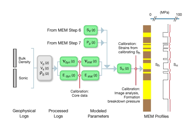
Step 9: Maximum Horizontal Stress Model

The profile of the maximum horizontal stress, $S_H$ , is often represented using the poroelastic strain model since it is calculated when using elastic strains to calibrate the $S_h$ profile. Figure 10 illustrates modeling $S_H$ using the poroelastic model.

This profile is normally calibrated to values of $S_H$ obtained from modeling wellbore deformation observed in borehole images. Occasionally the Hubbert and Willis breakdown equation is used to estimate $S_H$ when open hole stress measurements or leakoff tests are available. When elastic strains are used to calibrate the profile of $S_h$ , the equations of elasticity specify the magnitude of $S_H$ as well. So, an internally consistent stress model can only result when both $S_h$ and $S_H$ are calibrated simultaneously. To emphasize this point the $S_h$ profile is included as a dotted line in Figure 10.

An alternative method is to construct a depth trend for the $S_H$ -based least-squares and fit values of $S_H$ obtained by modeling wellbore damage. This approach is often used early in the life of a field when data are sparse.

Maximum Horizontal Stress Model, The Mechanical Earth Model MEM,Mechanical Earth Model,Geomechanics,Rock properties,Stress distribution,Strain,Elastic deformation,Plastic deformation,Shear strength,Fracture mechanics,Faults,Pore pressure,Rock mechanics,Reservoir simulation,Wellbore stability,Rock failure,Rock strength,Geotechnical analysis,Formation evaluation,Borehole stability,Rock behavior,Stress-strain relationship,Deformation analysis,Rock physics,Geostress,Mechanical properties,Mechanical Earth Model,Geomechanics,Geomechanical Analysis,Earth Model,Understanding Earth's Mechanics,Advanced Geomechanics,Mechanical Earth Model,Geomechanics,Earth Model,Geomechanical Analysis,Understanding Earth's Mechanics,Advanced Geomechanics,Earth Modeling Techniques,Geomechanical Properties,Mechanical Behavior of Earth,Geomechanical Modeling,Earth Stress Analysis,Introduction to Geomechanics,Earth Deformation Analysis,Geomechanical Engineers,Earth Material Properties,Geomechanical Testing,Earth Stress Modeling,Application of Geomechanics,Geomechanical Consultants,Earth Stability Analysis,Geomechanical Software,Earth Mechanics Principles — **Figure 10**: Modeling $S_H$ using the poroelastic model

Step 10: Stress Direction

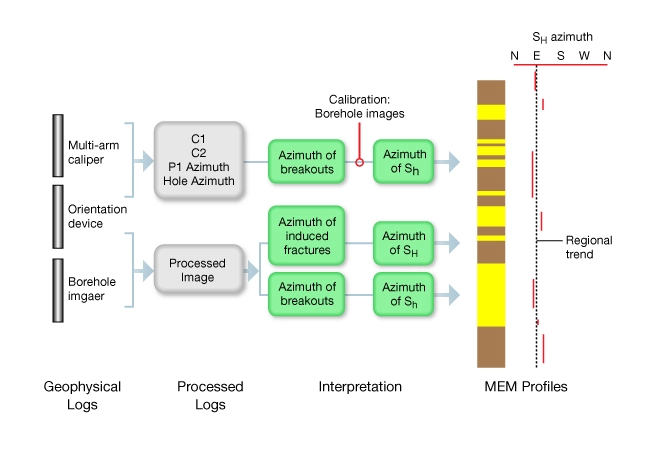
A stress direction profile can be generated at any time since it does not use inputs from other MEM profiles. However, you gain a deeper understanding of the regional geomechanics if done as Step 10. At the very least you should have a framework model (Step 2). Stress direction is obtained from the interpretation of wellbore damage measured either by oriented multi-axis caliper logs or borehole images. The caliper method provides an estimate of the least horizontal stress direction from interpretation of borehole elongations. The borehole image method is more accurate since the directions of $S_h$ and $S_H$ are determined from wellbore breakouts and drilling-induced extension fractures.

An internally consistent model shows that azimuths of $S_h$ and $S_H$ are orthogonal to one another. Stress direction is usually represented by a constant azimuth as a function of depth in the well. The azimuth is computed from a least-squares fit to stress direction data. If there is no definite trend or if the azimuth rotates with depth, this should be captured in the model. Figure 11 illustrates the two methods for constructing a stress direction profile.

Caliper-based interpretation methods are designed to differentiate stress-induced elongation from other sources of wellbore damage. However, it is recommended that the interpretation be checked using borehole images when possible. No calibration steps are shown for image analysis as this is the most direct method for determining stress direction.

Stress direction, The Mechanical Earth Model MEM,Mechanical Earth Model,Geomechanics,Rock properties,Stress distribution,Strain,Elastic deformation,Plastic deformation,Shear strength,Fracture mechanics,Faults,Pore pressure,Rock mechanics,Reservoir simulation,Wellbore stability,Rock failure,Rock strength,Geotechnical analysis,Formation evaluation,Borehole stability,Rock behavior,Stress-strain relationship,Deformation analysis,Rock physics,Geostress,Mechanical properties,Mechanical Earth Model,Geomechanics,Geomechanical Analysis,Earth Model,Understanding Earth's Mechanics,Advanced Geomechanics,Mechanical Earth Model,Geomechanics,Earth Model,Geomechanical Analysis,Understanding Earth's Mechanics,Advanced Geomechanics,Earth Modeling Techniques,Geomechanical Properties,Mechanical Behavior of Earth,Geomechanical Modeling,Earth Stress Analysis,Introduction to Geomechanics,Earth Deformation Analysis,Geomechanical Engineers,Earth Material Properties,Geomechanical Testing,Earth Stress Modeling,Application of Geomechanics,Geomechanical Consultants,Earth Stability Analysis,Geomechanical Software,Earth Mechanics Principles — **Figure 11**: Methods for constructing a stress direction profile

Step 10: Completed MEM

Completed Mechanical Earth Model, The Mechanical Earth Model MEM,Mechanical Earth Model,Geomechanics,Rock properties,Stress distribution,Strain,Elastic deformation,Plastic deformation,Shear strength,Fracture mechanics,Faults,Pore pressure,Rock mechanics,Reservoir simulation,Wellbore stability,Rock failure,Rock strength,Geotechnical analysis,Formation evaluation,Borehole stability,Rock behavior,Stress-strain relationship,Deformation analysis,Rock physics,Geostress,Mechanical properties,Mechanical Earth Model,Geomechanics,Geomechanical Analysis,Earth Model,Understanding Earth's Mechanics,Advanced Geomechanics,Mechanical Earth Model,Geomechanics,Earth Model,Geomechanical Analysis,Understanding Earth's Mechanics,Advanced Geomechanics,Earth Modeling Techniques,Geomechanical Properties,Mechanical Behavior of Earth,Geomechanical Modeling,Earth Stress Analysis,Introduction to Geomechanics,Earth Deformation Analysis,Geomechanical Engineers,Earth Material Properties,Geomechanical Testing,Earth Stress Modeling,Application of Geomechanics,Geomechanical Consultants,Earth Stability Analysis,Geomechanical Software,Earth Mechanics Principles — **Figure 12**: Completed MEM

Model Revision

Initial geomechanical models often are uncalibrated or the calibration is limited only to parts of the model. To maximize the benefit of geomechanics to a field asset, it helps to view geomechanical modeling as an iterative process. Figure 13 illustrates an iterative modeling workflow. The data audit and MEM building workflows are represented by the grey boxes. The iterative aspects of this workflow are represented by the red, green and yellow boxes. The key idea is to use the MEM to perform a geomechanics forecast, such as wellbore stability or hydraulic fracture design, and compare predictions of the forecast to field observations. If the prediction is validated, the model is adequate for operational purposes. If not, the discrepancies are analyzed until the sources of error are identified and the model is revised.

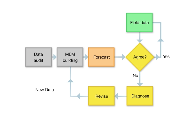
It is highly recommended that geomechanical models be revised as critical missing data or calibration data become available. Model revision can entail acquiring new data or simply improving calibration. Calibration of pore pressure, earth stress magnitudes, and better understanding of lateral variations in the rock mechanical properties are typical examples of model refinements.

Benefits of the Mechanical Earth Model

Improved Reservoir Characterization: The MEM enhances reservoir characterization by providing a detailed understanding of the mechanical properties of subsurface formations. It helps in identifying the stress distribution, rock strength, and elastic properties of reservoir rocks, which are critical for accurate reservoir modeling and simulation.
Enhanced Wellbore Stability Analysis: Wellbore stability is a significant concern in drilling operations. The MEM enables engineers to assess the stability of wellbores under different stress conditions. By understanding the mechanical behavior of the rocks surrounding the wellbore, operators can optimize drilling parameters and mitigate potential wellbore instability issues.
Optimized Hydraulic Fracturing: Hydraulic fracturing is a widely used technique to enhance reservoir productivity. The MEM aids in designing effective fracturing treatments by considering the in-situ stress regime, rock mechanical properties, and fluid flow behavior. It helps operators identify the optimal fracture orientation and placement for maximum reservoir contact and improved production rates.
Accurate Production Forecasting: The MEM contributes to accurate production forecasting by incorporating rock deformation and fluid flow properties. By considering the mechanical behavior of reservoir rocks, operators can assess the impact of production on reservoir compaction, subsidence, and fluid migration. This knowledge allows for more reliable predictions of long-term reservoir behavior and production decline rates.
Risk Mitigation: The MEM helps in mitigating risks associated with reservoir management operations. By understanding the stress distribution and rock strength, operators can identify potential areas of high-risk such as fault zones, weak formations, or regions prone to induced seismicity. This knowledge enables proactive measures to minimize risks and ensure safe and sustainable production.