Earth Stress | What is Earth stress?

50 minutes read

Stress-directions-from-shear-wave-anisotropy

Modeling Horizontal Stress

A geomechanical model of horizontal stress is a quantitative description of the variations of $S_h$ and $S_H$ with depth. While it represents the current knowledge of the contemporary stress at a specific location of interest, it does not describe the evolution of stress over geologic time.

In this section we present models that can be used to predict stress in a variety of geologic settings. We will see that models can account for observed variations of $S_h$ because lithology-dependent model parameters, vertical stress, and pore pressure are inputs to all the models.

We begin by describing two methods for modeling pore pressure. Next, we examine horizontal stresses that result from elastic and inelastic deformation under three different strain boundary conditions: uniaxial strain, plane strain, and triaxial strain. We conclude by calibrating the poroelastic model of $S_h$ in two different geologic settings and describing a method for calibrating the magnitude of $S_H$ using borehole images.

Pore Pressure Modeling

All geomechanical models require pore pressure in order to compute effective stress. Pore pressure models derive from geophysical methods used to detect and quantify pore pressure. Two of the most widely used methods to transform compressional wave velocity, $V_p$ , to $P_p$ are those of Eaton (1975) and Bowers (1995). Pressure prediction is routine, and most reliable, in settings where overpressure is due to compaction disequilibrium. Basins located on continental margins and other settings where rapid sedimentation has occurred are the best candidates for geophysics-based pore pressure prediction. It is much more difficult and less reliable to model pore pressure in rocks located in tectonically active regions. Modeling pressure in these regimes requires careful integration of drilling data, pressure measurements, basin modeling and geophysical measurements. In cases where data are extremely limited, hydrostatic pressure or mud weight used to drill nearby wells serves as a starting model for pore pressure.

Successful pore pressure prediction methods are rooted in observations of overpressure reported by Hottman and Johnson (1965). They demonstrated that in thick shale formations, resistivity and compressional wave velocity respond to variations in effective vertical stress, $\sigma _V$ . They showed that $P_p$ trends can be mapped given a measurement of effective stress (for example $V_p$ or $Dt_c$ or resistivity) and an estimate of the overburden stress, $S_V$ . From the definition of effective vertical stress:

$P_p = S_V - \sigma _v$

Where:

$S_V = g\, \displaystyle \int _{0}^{z} \rho _b(z)\, \mathrm{d}z$

Seismic and sonic velocity based methods for modeling pore pressure are preferred in geomechanics because:

They may be used with surface seismic data, borehole check shots, or sonic logs.
$V_p$ is relatively insensitive to temperature.
Pre-drill seismic-based predictions can be calibrated while drilling the first exploration well using LWD sonic, check shots, and wireline data.

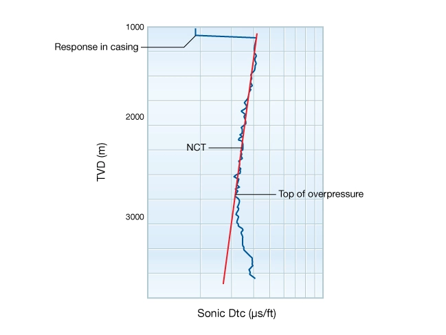
Figure 1 shows a schematic sonic log through thick shale, crossing from a normally pressured section to an overpressured section. In subsiding basins, the top of overpressure is easily detected, as is shown here. However, this is not true when pressures develop after the rock has lithified.

Sonic-log-through-shale — **Figure 1**: Sonic log through shale

Eaton’s Method

Eaton’s velocity method is given by the formula:

$\sigma_{_{V}}=\sigma_{norm}\left ( \dfrac{V_p}{V_{norm}} \right )^3$

Where:

$\sigma_{norm}$ is the effective vertical stress corresponding to hydrostatic pore pressure

$V_p$ is the measured compressional wave velocity

$V_{norm}$ is the velocity in normally pressured shale

Figure 1 shows a normal compaction trend (NCT) line in red. Referring to Eaton’s equation, $V_p = V_{norm}$ along the normal trend line. Shale is presumed to be overpressured when $V_p$ is less than $V_{norm}$ (or $Dt_c$ is greater than $Dt_{cnorm}$ ). Pore pressure is then calculated given a measure of the vertical stress:

$P_p = S_V - \sigma_{_{V}}$

Eaton’s method is calibrated to pressure measurements by adjusting the normal compaction trend or by varying the exponent from its starting value of 3, or both. Normal compaction trends tend to be clearly defined in young, subsiding basins but less so in well-compacted sections or ones which have been tectonically uplifted. Establishing a normal compaction trend is the main challenge with this method.

Bowers’ Method

Bowers’ method does not require a normal compaction trend but it does require a model of $ Vp $ as a function of effective stress. The form of the Bowers’ velocity model is:

$V_p=V_0 + A\, \sigma_{_{V}}^B$

where $V_0$ is the velocity of the unstressed fluid-saturated sediment, and A and B are model parameters describing the variation of velocity with effective stress. It follows that:

$\sigma _{_{V}}=\left [ A^{-1}\left ( V_p-V_0 \right ) \right ]^{B^{-1}}$

and so

$P_p = S_V - \sigma_{_{V}}$

Bowers’ method applies whether the effective stress increases during compaction (loading path), or decreases after rocks have lithified (unloading path) due to fluid expansion. The unloading path describes situations when hydrocarbons are generated after the rock has lithified or the pore fluids are heated (aquathermal pressuring). Figure 2 illustrates these two loading paths.

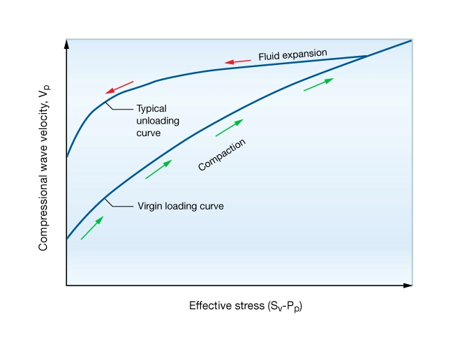
Loading-vs-unloading-paths-of-Bowers-method — **Figure 2**: Loading vs. unloading paths of Bowers method

Notice that the slope of the unloading curve is less than that of the loading curve, except at very low effective stress. This indicates that $V_p$ is less sensitive to pore pressures generated by aquathermal pressuring, hydrocarbon maturation or tectonic uplift.

For engineering applications, both the Eaton and Bowers method require calibration. Calibration may be achieved using drilling mud weights, reports of losses or kicks, or direct pressure measurements made while drilling a well.

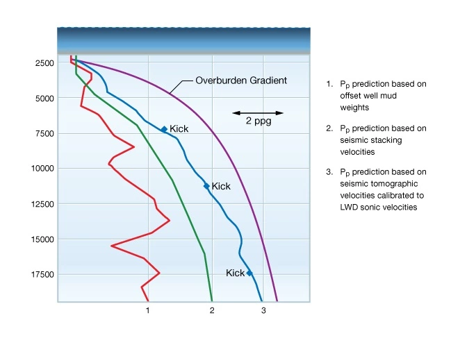
Figure 3 shows a comparison of the uncertainty possible in three pre-drill pore pressure predictions.

Curve 1 is a prediction based on mud weights used to drill offset wells.

Curve 2 is a prediction based on seismic stacking velocity.

Curve 3 was obtained using a tomographic velocity analysis of the same seismic data used to generate curve 2 and calibrating to LWD velocity measurements while drilling, and is the most accurate model. The predicted pressure based on the calibrated velocity was very close to the actual pressure as evidenced by the pressure signals “kicks” observed while drilling the well.

Pore-pressure-uncertainties — **Figure 3**: Pore pressure uncertainties

Uniaxial Strain Models

Uniaxial strain describes situations where rock deforms in the vertical direction (z) but not laterally: $\varepsilon _z \neq 0$ , $\varepsilon _x = \varepsilon _y = 0$ . The uniaxial consolidation model can be used to describe compacting sediments near the seafloor in marine environments. The uniaxial poroelastic model can be used to represent lithified sediments in tectonically inactive settings. Note that under uniaxial strain boundary conditions, gravitational loading and rock temperature are the only sources of stress, and that both horizontal stresses are equal.

Consolidation Model of Uniaxial Strain

The uniaxial consolidation model is commonly used in soil mechanics to model horizontal stress in laterally-confined sediments undergoing compaction:

$\sigma _h = K_0 \, \sigma _{V}$

$\sigma _H = \sigma _h$

Where:

$\sigma _h$ and $\sigma _{V}$ are the horizontal and vertical effective stresses, respectively

$K_0$ is the coefficient of earth stress measured in the laboratory

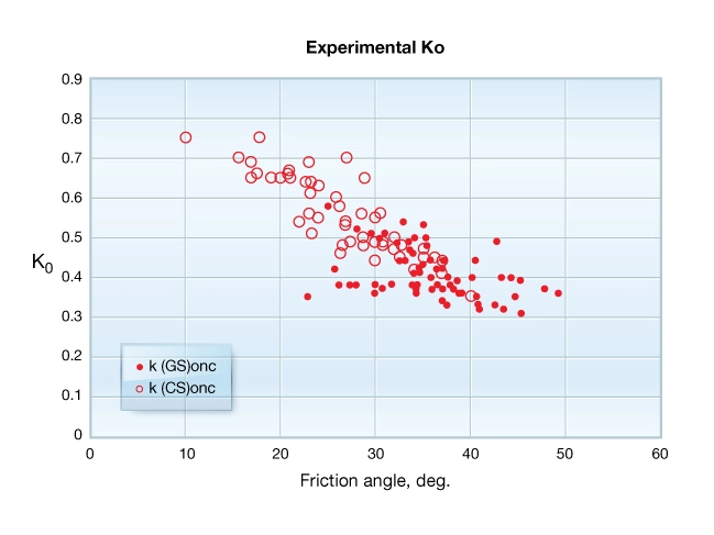
This model is appropriate for high-porosity, uncemented sediments with porosity greater than around 30%. Laboratory measurements show that $K_0$ varies with lithology, the degree of consolidation, and rock fabric. Figure 4 shows values of $K_0$ measured on sediments from the Gulf of Mexico. This figure illustrates a dependence on clay content and texture as inferred from friction angle. The statistical model for $K_0$ measured on clays is 0.65 and for sands it is 0.38. In these sediments, horizontal stress is predicted to range from $\sigma _h =$ 0.38 to 0.65 times $\sigma _V$ , where stress in the clay-rich mudrocks is predicted to be greater than for adjacent sands.

Coefficient-of-earth-stress-measurements — **Figure 4**: Coefficient of earth stress measurements in the Gulf of Mexico

Poroelastic Model of Uniaxial Strain

The horizontal effective stress in isotropic-poroelastic rock deforming under uniaxial strain boundary conditions is given by:

$\sigma _h = \dfrac{\nu}{1 - \nu}\sigma _V$

$\sigma _H = \sigma_h$

Where:

$\sigma _h$ and $\sigma _V$ are as defined for the consolidation model

$\nu$ is Poisson’s ratio

Consider a clay-free sandstone with Poisson’s ratio equal to 0.25. The effective horizontal stress is predicted to be $\sigma _h = 13\, \sigma _V$ . For a mudstone or a shale with Poisson’s ratio of 0.4, $\sigma _h$ is predicted to be 23 $\sigma _V$ . Notice that both the uniaxial consolidation and poroelastic models predict higher horizontal stress in the clay-rich lithologies. This is a consequence of correlation between rock properties $K_0$ and $\nu$ , not to the boundary condition or deformation process.

Thermal Stress Model

Thermal stress can be a significant component of the horizontal stress in deep, high-temperature formations and in reservoirs where steam is injected. Thermal stresses develop in rocks when the free thermal expansion is prevented by lateral confinement. Heating or cooling a laterally confined isotropic rock induces a thermal stress, $\sigma _T$ , given by the expression:

$\sigma _T = \dfrac{\alpha _T\, E}{1-\nu}\, \Delta T$

Where:

$\alpha _T$ is the coefficient of linear thermal expansion

$\Delta T$ is temperature change

$E$ and $\nu$ are defined as Young’s modulus and Poisson’s ratio respectively

For sedimentary rocks the coefficient of linear thermal expansion ranges from about 8×10⁻⁶ to 15×10⁻⁶/deg. C. Notice that induced thermal stresses are proportional to Young’s modulus. So, for a given change in temperature, induced thermal stresses are greater in the stiffer rocks.

For example, consider the thermal stress difference between sandstone with 5% porosity and one with 20% porosity due to a 10 °C change in temperature. Table 1 shows that thermal stress can be significant and that bed-to-bed differences in Young’s modulus can result in significant thermally-induced stress contrasts.

Table 1: Comparison of Thermal Stresses Induced in Laterally Confined Sandstone with Different Physical Properties
	Porosity %	$\alpha_T$ 1/deg. C	$E$ GPa	$\nu$	$\Delta_T$	$\alpha_T$ MPa
Sandstone 1	5	12 $\times$ 10^-6	62	.15	10	8.75
Sandstone 2	20	15 $\times$ 10^-6	17	.25	10	3.4

Oilfield operations that may generate significant thermal stresses include circulation of cool drilling fluid in high temperature wells or injection of steam into heavy oil reservoirs.

Plane Strain and Triaxial Strain Models

Plane strain and triaxial strain boundary conditions apply to tectonically active settings where rock can deform in both horizontal and vertical directions. If one of the horizontal principal strains is equal to zero, and the other two are non-zero, the rock deforms in a state of plane strain. If all three principal strains are non-zero, the rock deforms in a state of triaxial strain. Under these conditions, sources of stress include gravitational loading and tectonic stress. Consequently, both boundary conditions lead to unequal horizontal stresses. This contrasts with deformation under uniaxial strain where only vertical deformation occurs and horizontal stresses are equal including gravitational loading and tectonic strain.

Poroelastic Model of Plane Strain

Consider an isotropic, poroelastic rock deforming in plane strain. This is the situation when a tectonic strain is acting in one horizontal direction and the rock is laterally restrained in the orthogonal direction that is, $\varepsilon _H$ and $\varepsilon _V \neq 0$ , $\varepsilon _h = 0$ . The horizontal stresses are given by:

$\sigma _h = \dfrac{\nu}{1-\nu}\, \sigma _{_{\!V}} + \dfrac{\nu\, E}{1-\nu^2}\varepsilon _H$

$\sigma _H = \dfrac{\nu}{1-\nu}\sigma _{_{\!V}}+\dfrac{E}{1-\nu^2}\varepsilon _H$

Notice that $\varepsilon _H$ contributes to both horizontal stresses. Compared to the uniaxial elastic strain model, the additional term $\frac{E \varepsilon _H }{1-\nu^2}$ represents the tectonic stress due the strain $\varepsilon _H$ . The term, $\frac{\nu E \varepsilon _H }{1-\nu^2}$ represents the component of tectonic stress, induced in the minimum horizontal stress direction by the Poisson effect.

Under conditions of triaxial strain, all principal strains are non-zero and the horizontal stresses are given by:

$\sigma _h = \dfrac{\nu}{1-\nu}\sigma _{_{\!V}} + \dfrac{E}{1-\nu^{2}}\varepsilon _h + \dfrac{\nu E}{1-\nu^2}\varepsilon _H$

$\sigma _H = \dfrac{\nu}{1-\nu}\sigma _{_{\!V}} + \dfrac{E}{1-\nu^{2}}\varepsilon _H + \dfrac{\nu E}{1-\nu^2}\varepsilon _h$

Notice that both horizontal stresses contain $\varepsilon _H$ and $\varepsilon _h$ terms. Since the strains cannot be measured in-situ, they are used for calibration. They permit this model to fit to a wide range of measured stress profiles.

The preceding discussion pertains to isotropic elastic rocks. However, some sedimentary rocks, particularly shales, are known to be elastically anisotropic.

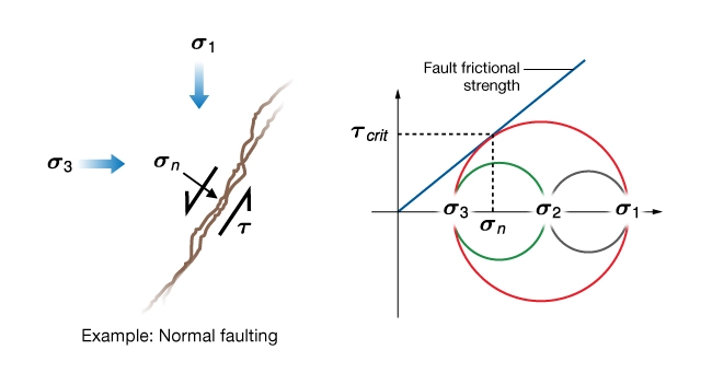
Frictional Equilibrium Model

It has long been argued that rock strength limits the magnitude of shear stress in the earth’s crust. One such hypothesis is that the maximum shear stress is governed by the frictional strength of favorably oriented faults. Frictional sliding is an inelastic process that occurs under plane strain or triaxial strain boundary conditions. The concept is that once the shear stress on a fault reaches the frictional strength, the fault slips, and the shear stress drops. Subsequent tectonic loading may lead to an increase in the shear stress up to the frictional strength at which point the fault again slips. Thus, the shear stress on the fault can never exceed a critical value. This is called the frictional equilibrium hypothesis and is express by the formula:

$\dfrac{\sigma _{1}}{\sigma _{3}} = \left [ \left ( \mu ^2 + 1 \right )^{\left( \frac{1}{2} \right)}+\mu \right ]^{2}$

Coefficient-of-fault-friction — **Figure 5**: Coefficient of fault friction

In practice, the frictional equilibrium model is used early in the life of a field when no direct measurements have been made. Horizontal stresses are calculated using estimates of $S_V$ and $P_p$ derived from seismic data and assuming Byerlee’s law applies ( $\mu$ = 0.85). However, some researchers allow $\mu$ to range between 0.6 and 1.0. This range of values allows this model to fit many of the measured depth trends of $S_h$ but not the bed-to-bed variations shown in Figure 6.

Multi-basin-comparison-of-stress-ratio — **Figure 6**: Multi-basin comparison of stress ratio

The frictional equilibrium model predicts a lower bound on $S_h$ and an upper bound on $S_H$ . This is because a decrease in $S_h$ or an increase in $S_H$ would result in an increase in shear stress, which by definition, is limited by the frictional strength of the faults. So strike-slip faults causes the effective stress ratio to remain constant.

Expressing the frictional equilibrium model in terms of measureable stresses leads to constraints on either the minimum or the maximum principal horizontal stress. For a normal faulting regime the model predicts a lower bound on $S_h$ :

$S_h = \left ( S_V - P_p \right )\left [ \left ( \mu ^2 + 1 \right )^{\left( \frac{1}{2} \right)} + \mu \right ]^{-2} + P_p$

For a thrust faulting regime, the model predicts an upper bound on $S_H$ :

$S_H = \left ( S_V - P_p \right )\left [ \left ( \mu ^2 + 1 \right )^{\left( \frac{1}{2} \right)} + \mu \right ]^{2} + P_p$

Given a measurement of $S_h$ in a strike-slip faulting regime, the model provides an upper bound on $S_H$ :

$S_H = \left ( S_h - P_p \right )\left [ \left ( \mu ^2 + 1 \right )^{\left( \frac{1}{2} \right)} + \mu \right ]^{2} + P_p$

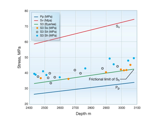
Bounds on the horizontal stresses may be calculated using measurements of $S_h$ , $S_V$ , $P_p$ , and assuming a value for $\mu$ . Figure 7 compares the bounds on $S_h$ and $S_H$ predicted for normal and thrust faulting regimes to the hydrostatic and lithostatic reference states. Bounds were calculated assuming $\mu$ = 0.85, $P_p$ = 10.5 MPa/km, and $S_V$ = 22.6 MPa/km. Shown for comparison is the uniaxial strain model prediction for $S_h$ assuming a Poisson’s ratio of 0.25.

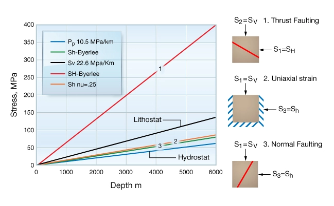
Comparison-of-horizontal-stresses-in-normal-vs-thrust-faulting — **Figure 7**: Comparison of horizontal stresses in normal vs. thrust faulting

Figure 8 compares a prediction of $S_h$ , assuming normal faults are in frictional equilibrium, to stresses measured in a well. This prediction was computed using measured pore pressure, vertical stress computed by integrating formation bulk density, and assuming $\mu$ = 0.85. Note that the frictional limit predicts the lower bound to the measured stresses but it does not predict the lithology dependent stress.

Comparison-of-horizontal-stress — **Figure 8**: Comparison of horizontal stress to the actual well data

Calibrating Stress Models

We conclude this section by illustrating how stress models may be calibrated to in-situ measurements. First we calibrate the poroelastic model of $S_h$ in two distinctly different geologic settings the East Texas basin and the Appalachian plateau. Then we describe a method to calibrate the magnitude of $S_H$ using borehole images and previously calibrated geomechanical parameters.

In East Texas, measurements of $S_h$ are consistent with the uniaxial strain boundary condition. On the Appalachian plateau, a plane strain model is required to match the measured stress profile. Figure 9 shows a schematic diagram of stress profiles represented by these two examples. In East Texas, $S_h$ is greater in shale than in adjacent sandstone. On the Appalachian plateau, the situation is reversed and stress in shale is less than in sandstone or limestone.

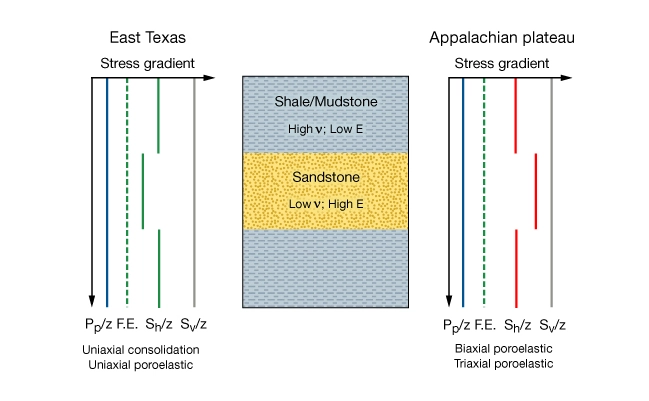
Schematic-stress-profiles-for-East-Texas — **Figure 9**: Schematic stress profiles for East Texas and the Appalachian plateau

These two examples highlight an important point for reservoir stimulation by hydraulic fracturing. Horizontal stress does not always increase with Poisson’s ratio as is often assumed in hydraulic fracture designs. The contemporary horizontal stress depends both on rock mechanical properties and the current boundary conditions. In one case $S_h$ is proportional to Poisson’s ratio, in another case it is the reverse. The only way to detect stress profiles like the Appalachian example is to measure stress in both shale and adjacent reservoir sandstone or limestone.

A stress profile is considered calibrated if it:

Matches the depth trend of the measured stress magnitudes.
Honors the pore pressure trends.
Honors lithology dependent trends.
Is consistent with current rock deformation mechanisms.

Calibrating $S_h$ in the East Texas Basin

This example features twenty-six cased-hole hydraulic fracturing stress measurements made in a well, located in the East Texas basin. The well penetrates the Lower Cretaceous Travis Peak formation, a sequence of sandstone, siltstone, and shale. Figure 8 shows the variation of $S_h$ measured over a depth interval of 700 m. Shown for reference is the overburden stress, pore pressure, and $S_h$ predicted by the frictional equilibrium model. Notice that $S_h$ measured in sandstone $S_s$ is systematically less than that measured in adjacent shale formations $S_h$ . Stress in siltstone ( $S_{lt}$ ) is intermediate between the other lithologies.

Key features of this data set to be captured by this stress model are:

Stress and pore pressure increases with depth.
Stress magnitude is systematically greater in rocks with high clay content.

The first step in constructing the stress profile is to select one of three reference models. The frictional equilibrium model is rejected because it does not predict lithology dependent stress. The uniaxial consolidation model is rejected because the rocks are low porosity ( $\sim$ 6%) and are well cemented. This leaves the poroelastic model to consider.

$\sigma _h = \dfrac{\nu}{1-\nu}\sigma _V$

If this model is appropriate and if uniaxial strain boundary conditions apply, the measured stress should be proportional to Poisson’s ratio. Figure 10 shows this is the case. Notice that stress increases with increasing Poisson’s ratio.

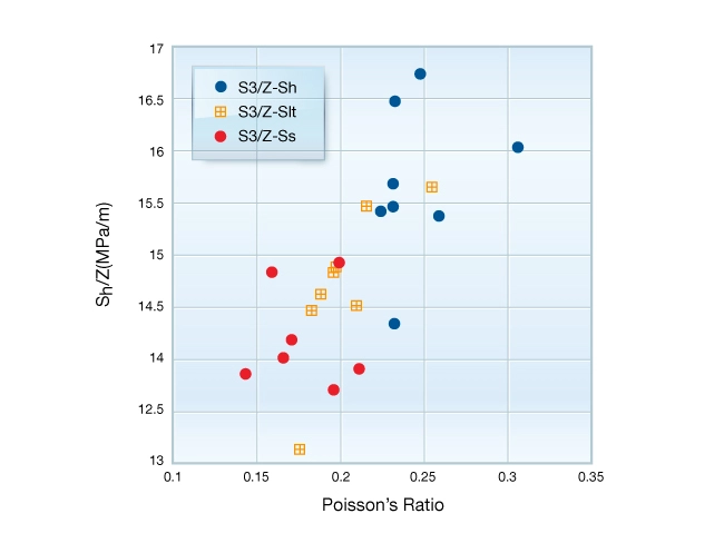
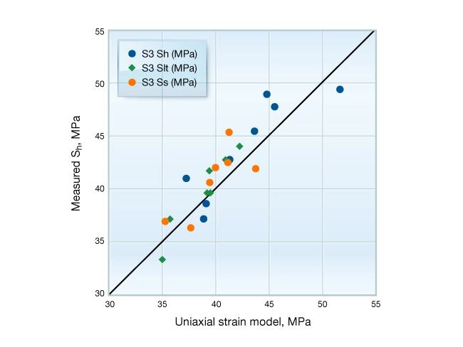
Horizontal-stress-related-to-Poisson-ratio — **Figure 10**: Horizontal stress related to Poisson’s ratio

Figure 11 compares measured stress to stress predicted by the poroelastic model assuming uniaxial strain boundary condition. The match is very good using only log-derived values of Poisson’s ratio, a profile of $S_V$ computed from a density log and a pore pressure profile calibrated to three reservoir pressure measurements. The symmetric scattering of points around the 1:1 correlation line indicates the model predicts the measured stress to within a few MPa. Thus, at this location, the measured stress profile is consistent with the uniaxial poroelastic model.

Measured-vs-predicted-stress — **Figure 11**: Measured vs. predicted stress in a poroeleatic model

Calibrating $S_h$ on the Appalachian Plateau

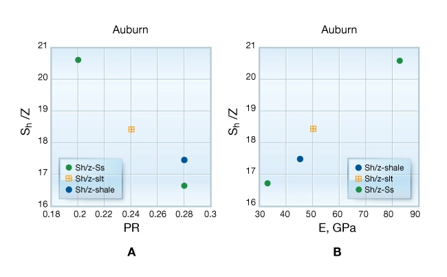
This example features a research well drilled on the Appalachian Plateau at Auburn, New York. The well penetrates low-porosity Paleozoic carbonates, sandstones, and shales. The area is well known for its shallow-focus intraplate earthquakes and a regional $S_H$ oriented ENE-WSW. Four open-hole hydraulic fracture stress measurements were made over a depth interval of 1000 m. Given the age and porosity of these sediments, it is appropriate to try to calibrate the stress profile to a poroelastic model. However, Figure 12 A shows that $S_h$ is negatively correlated with Poisson’s ratio, unlike the East Texas example. Also notice that $S_h$ measured in the high Poisson’s ratio shale is low compared to the two other measurements.

These observations are inconsistent with a uniaxial strain boundary condition, indicating that gravitational loading only accounts for part of the horizontal stress here. Instead, $S_h$ is correlated to Young’s modulus (Figure 12 B). A correlation with Young’s modulus suggests that either thermal stress,

$\sigma _T = \dfrac{\alpha _T\, E}{1 - \nu}\Delta T$

or tectonic stress,

$\sigma _{tectonic}=\dfrac{\nu\, E}{1 - \nu^{2}}\varepsilon _H$

contributes to the measured stress here.

Calibration-of-the-poroelastic-model — **Figure 12**: Calibration of the poroelastic model

In the absence of core data or temperature measurements, the simplest model that includes a dependence on Young’s modulus and is consistent with the contemporary tectonic setting is tried. Given that the region is still rebounding from the last glaciation and that it is tectonically active, a thermal stress source is rejected in favor of a tectonic source. The simplest solution is to invoke a plane strain model with compressive tectonic strain acting in the direction of $S_H$ . Therefore, least horizontal stress is modeled as:

$\sigma _h = \dfrac{\nu}{1 - \nu}\sigma _{_{\!V}}+\dfrac{\nu E}{1-\nu^{2}}\varepsilon _H$

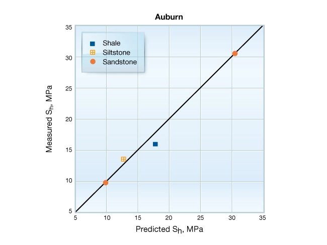
Figure 13 shows the plane strain poroelastic stress model is well calibrated using a constant horizontal strain gradient over the 1 km depth interval. Again, the calibrated model shows only that the measured $S_h$ is consistent with this model, not that the model explains the origin of stress. The calibrated model indicates that gravitational loading alone does not account for the observed stress profile and that shales, in this case, are not expected to act as barriers to hydraulic fracture propagation.

Plane-strain-poroelastic-model — **Figure 13**: Plane strain poroelastic model

Calibrating $S_H$

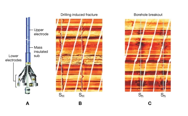
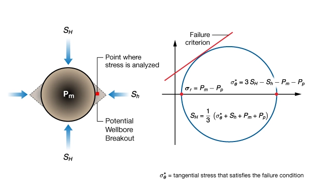
We have seen how models of the least horizontal stress may be calibrated to hydraulic stress measurements. Although models of $S_H$ cannot be calibrated to direct measurements, it is possible to constrain the magnitude of $S_H$ by calculating the hoop stress required to create wellbore breakouts observed in borehole images shown in Figure 14 B and Figure 15 C. This approach is used to constrain the horizontal strain terms used to calibrate poroelastic models described previously.

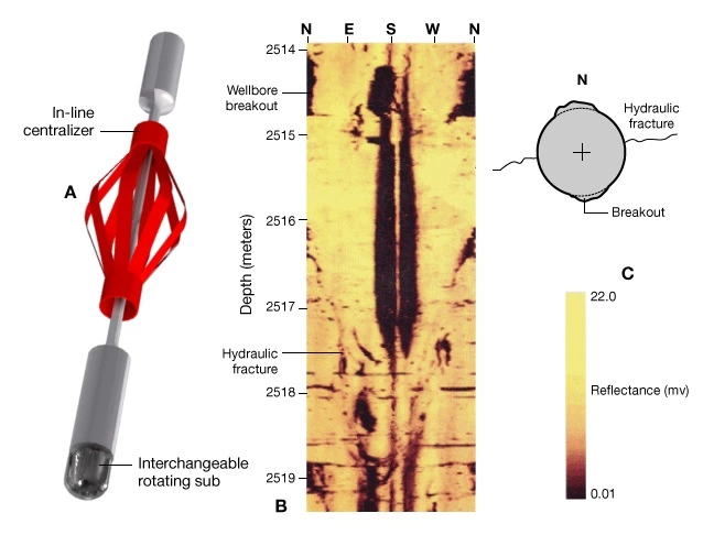
acoustical-imaging-tool-UBI — **Figure 14**: Acoustical imaging tool

electrical-imaging-tool-FMI — **Figure 15**: Electrical imaging tool

The method requires a borehole image showing wellbore breakout plus values of $P_p$ , $S_h$ , $S_V$ and rock strength for those intervals. This is normally the last step in an earth stress analysis since it depends on developing a considerable amount of input data.

The method is illustrated in Figure 16. Consider a small element of rock located adjacent to the wellbore surface at the azimuth of $S_h$ ( $\theta =$ 90). Breakouts initiate here when the hoop stress equals the compressive strength of the rock, $\sigma_f^*$ . The critical hoop stress is given by:

$\sigma _{\theta \ (\theta = 90)} = \sigma _f^*$

Expanding $\sigma _{\theta }$ in terms of the far field stresses gives:

$\sigma _f^* = 3S_H - S_h - P_m - P_p$

Solving for $S_H$ :

$S_H =\dfrac{1}{3}( \sigma _f^* +S_h + P_m + P_p)$

Where:

$\sigma _f^*$ is the compressive strength of the rock

$P_m$ is the mud pressure in the well

$P_p$ is the formation pore pressure

These equations are simplified to illustrate the concept. In practice, numerical modeling is required to obtain more accurate results.

Calibrating-horizontal-stress — **Figure 16**: Calibrating horizontal stress

This method provides lithology-dependent estimates of $S_H$ through the lithology dependence on $\sigma _f^*$ and $S_h$ . The best estimate of $S_H$ is obtained where initial breakouts are imaged. That is where no caliper anomaly exists, just fractures visible in the image. A lower bound on $S_H$ is obtained in intervals where breakouts are well developed and produce a well-defined caliper anomaly.

By analogy, the magnitude of $S_H$ is also constrained by modeling the hoop stress required to generate drilling-induced hydraulic fractures. In intervals where neither breakouts nor drilling induced fractures are observed, an upper bound on $S_H$ may be calculated.