Earth Stress | What is Earth stress?

50 minutes read

Stress-directions-from-shear-wave-anisotropy

Borehole Measurements

Establishing the regional stress regime helps to reduce uncertainty about the state of stress for a specific location. But the best information comes from direct borehole measurements. This section discusses borehole measurements of stress direction, stress magnitude, and pore pressure. These data provide the calibration to stress models developed later in the module.

The most useful datasets are from deep boreholes drilled to access hydrocarbons or for scientific research. We begin by exploring how borehole stress concentrations make it possible to measure stress deep in the earth. Then we review borehole-imaging technology used to detect and map stress-induced features on the wellbore. Finally, this information is combined to show how the principal stress direction, magnitudes and pore pressure are measured downhole.

Borehole Stress Concentrations

The existence of borehole stress concentrations makes it possible to measure stress magnitude and stress direction deep in the earth. Miles and Topping (1949) applied the Kirsch solution for stresses around a circular hole in a stressed plate to describe the stress concentration around boreholes drilled into a stressed earth. The stress field near the surface of a borehole, drilled into a homogeneous elastic formation, subject to far-field stress, $S_H$ , is given in polar coordinates by:

$\sigma_{r}=\frac{S_{H}}{2}\left(1-\frac{R^{2}}{r^{2}}\right)+\frac{S_{H}}{2}\left(1+3 \frac{R^{4}}{r^{4}}-4 \frac{R^{2}}{r^{2}}\right) \cos 2 \theta$

$\sigma_{\theta}=\frac{S_{H}}{2}\left(1+\frac{R^{2}}{r^{2}}\right)-\frac{S_{H}}{2}\left(1+3 \frac{R^{4}}{r^{4}}\right) \cos 2 \theta$

$\tau_{r \theta}=\frac{S_{H}}{2}\left(1-3 \frac{R^{4}}{r^{4}}+2 \frac{R^{2}}{r^{2}}\right) \sin 2 \theta$

Where:

$S_H$ is the maximum horizontal stress.

$R$ is the radius of the borehole.

$r$ is the distance measured radially from the center of the hole.

$\theta$ is the angle measured clockwise from the azimuth of $S_H$ .

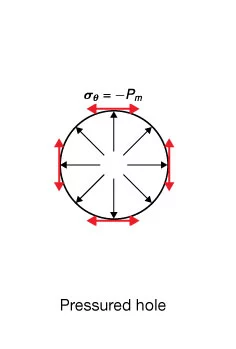
Inspection of these equations shows that there are four stress concentrations, localized at the borehole surface. Two are at the azimuth of the applied stress, $\theta$ = 0 and 180 degrees, and the others are at $\theta$ = 90 and 270 degrees (Figure 1 A). A few borehole diameters away from the wellbore, the “far-field” stresses are unaffected by the presence of the borehole. For the purpose of this discussion it should be understood that identical stress concentrations exist in diametrically opposed positions. Therefore, only those at $\theta$ = 0 and $\theta$ = 90 degrees are discussed. The mechanical basis for borehole stress measurements can be understood by observing how the hoop stress ( $\sigma_{\theta}$ ) is affected by borehole fluid pressure ( $P_w$ ) and the biaxial far-field stress ( $S_H$ and $S_h$ ).

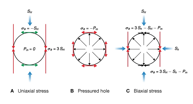**Figure 1**: Contributions to the hoop stress in a vertical wellbore aligned with a principal stress: A) hoop stress induced by a uniaxial far-field stress, $S_H$ ; B) hoop stress induced by a uniform well pressure; C) superposition of biaxial far-field stresses, $S_H$ and $S_h$ , and well pressure

Contributions to Hoop Stress

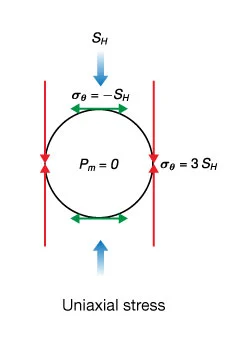
Uniaxial Far-Field Stress

Consider a borehole drilled into a formation subjected to a uniaxial far-field stress $S_H$ oriented at $\theta = 0$ . At the surface of an air-filled borehole, the radial stress $\sigma _r = 0$ and the hoop stress is:

$\sigma_{\theta (r = R, \theta)} = S_H - 2 S_H \cos{2 \theta}$

The hoop stress at the azimuth of the applied stress ( $\theta = 0$ ) is tensile and equal in magnitude to the applied stress

$\sigma_{\theta (r = R, \theta = 0)} = - S_H$

and at $\theta = 90$ degrees, it is compressive and equal to three times the applied stress

$\sigma_{\theta (r = R, \theta = 90)} = 3S_H$

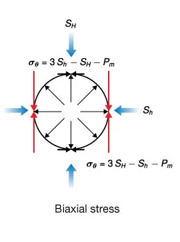
In general, $S_h$ is not zero, so the contribution of $S_h$ to the hoop stress concentration is obtained by linear superposition of $S_h$ in the orthogonal direction. Thus for a biaxial stress field, the hoop stress at $\theta = 0$ becomes:

$\sigma_{\theta (r = R, \theta = 0)} = -S_H + 3 S_h$

and $\theta = 90$ degrees becomes:

$\sigma_{\theta (r = R, \theta = 90)} = -S_h + 3 S_H$

Uniaxial-Far-Field-Stress — Uniaxial Far-Field Stress

Uniform Well Pressure

Now consider the contribution to the hoop stress from pore pressure inside the borehole pressure. Borehole pressure, due to the presence of drilling mud, ( $Pm$ ) induces a uniform tensile stress at all angles around the wellbore:

$\sigma_{\theta (r = R, \theta)} = -P_m$

Uniform-Well-Pressure — Uniform Well Pressure

Superposition of Biaxial Far-Field Stresses and Well Pressure

Superposition of all three stresses leads to equations widely used to interpret borehole stress measurements and borehole images. The hoop stress at the azimuth of the maximum horizontal stress, $SH$ , $\theta = 0$ is:

$\sigma_{\theta (r = R, \theta = 0)} = -S_H + 3S_h - P_m$

and the hoop stress at the azimuth least horizontal stress, $Sh$ , at $\theta = 90^{\circ}$ , is:

$\sigma_{\theta (r = R, \theta = 90)} = -S_h + 3S_H - P_m$

Biaxial-Far-Field-Stress — Superposition of Biaxial Far-Field Stresses and Well Pressure

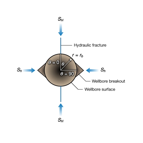
As a consequence of borehole stress concentrations, hydraulically induced fractures (tensile failure) develop preferentially at $\theta$ = 0 and 180 degrees relative to the maximum horizontal stress. Wellbore breakouts (compressive failure) develop at $\theta$ = 90 and 270 degrees. This explains why the contemporary stress direction can be determined using wellbore images. These features and their relationship to the far-field stresses are shown schematically in Figure 5. Note that this diagram of a borehole cross-section shows the relationship between stress-induced hydraulic fractures and wellbore breakout and the far field earth stresses, $S_H$ and $S_h$ . As we see here, $S_V$ is a principal stress.

Stress-induced-hydraulic-fractures-vs-borehole-breakout — **Figure 5**: Stress induced hydraulic fractures vs. borehole breakout

Borehole Imaging

Borehole images are a valuable source of geomechanics information. They are used to detect and map stress-induced wellbore damage, map geologic structures, and aid in the measurement of stress direction and stress magnitudes. This section reviews borehole image interpretation and how images are made.

Image Interpretation

A borehole image is constructed by flattening a cylindrical picture of the inside of a borehole (Figure 3). Imagine that a cylindrical picture of the inside of a well is cut at the azimuth, corresponding to North, $\theta$ = 0, and then flattened.

Theta is measured clockwise from North, so South ( $\theta$ = 180 degrees) is at the center of the image. In a deviated well the vertical edge of the image is normally set to the high side (top) of the hole. The radius $r$ is normally assumed to be constant and is set to one half of the drill bit diameter, and $z$ is depth measured along the axis of the well. Geologic features and wellbore damage are mapped using borehole image analysis software (Plumb and Luthi, 1986).

Borehole Image Schematics

Figure 6 depicts a vertical well intersecting a dipping plane, such as a bedding plane or a natural fracture.

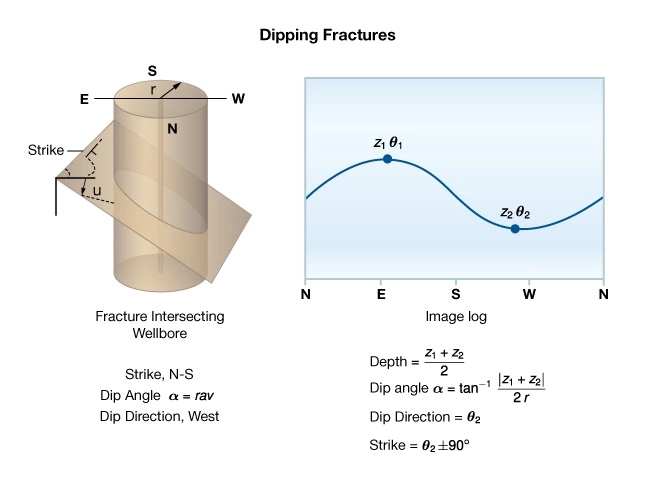
Constructing-a-borehole-image-of-dipping-fractures — **Figure 6**: Constructing a borehole image of dipping fractures

Figure 7 depicts the image of a vertical plane intersecting the hole across its diameter. This is an idealized image of how a hydraulic fracture would appear, where the traces of the fracture are separated by 180 degrees. A vertical natural fracture would also appear as two parallel lines but the traces would generally be separated by less than 180 degrees.

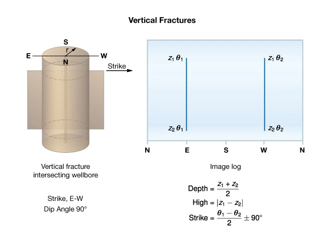
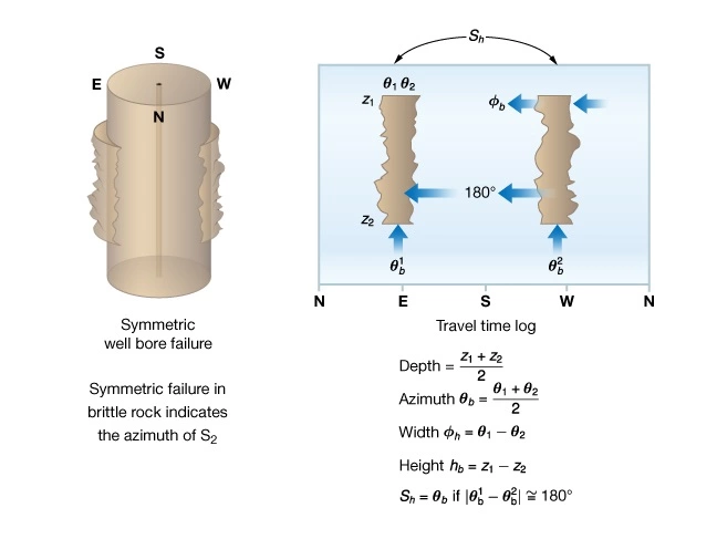
Constructing-a-borehole-image-of-vertical-fractures

Figure 8 shows how wellbore breakouts would appear in images. Each image shows how the feature can be mapped by recording the coordinates ( $\theta, z$ ) of key points on the image. More sophisticated algorithms are used in commercial image interpretation software to account for variations in borehole diameter with depth and borehole deviation. The examples shown here are meant to illustrate the concepts and only apply to vertical wells aligned with a principal stress.

Constructing-a-borehole-image-of-breakouts — **Figure 8**: Constructing a borehole image of breakouts

Imaging Tools

The majority of wellbore images are generated from acoustic or electric signals recorded by logging tools as they move along the axis of the hole. Less common are images formed from measurements of reflected light, bulk density, and gamma rays. Optical devices offer the highest resolution but only work in clear borehole fluids or in air-filled holes. Consequently, they are not practical in deep wells. Density and gamma ray images have much lower vertical and azimuthal resolution compared to images generated by acoustic or electrical signals.

Acoustic Tools

The first wellbore imaging tool was invented by the Mobil Oil Company in the late 1960s (Zemack and Caldwell, 1969). It was an acoustic device called the borehole televiewer (BHTV). Acoustic methods employ a rotating ultrasonic transducer that emits and receives a pulse of ultrasonic energy. Reflected amplitude and two-way transit time are measured for each ultrasonic pulse. The transducer fires about 180 times per revolution, although this number varies with tool manufacturer. Two 360-degree coverage images can be produced from this device:

A two-way transit time image measuring the borehole cross-section shape
A reflected amplitude image mapping acoustic impedance and/or surface roughness; dark areas of the image correspond to low acoustic impedance and/or rough surfaces; bright areas represent high acoustic impedance or a smooth surface

Acoustic images detect large-scale features such as wellbore breakouts, faults, relatively large natural fractures, and prominent contacts between lithologic units. They are most useful in the study of geomechanics and structural geology because they emphasize large-scale structures, but at the expense of small-scale sedimentological structures. A disadvantage of acoustic devices is that the performance degrades in wells filled with heavy drilling fluids (such as mud density of about 15 pounds per gallon or greater).

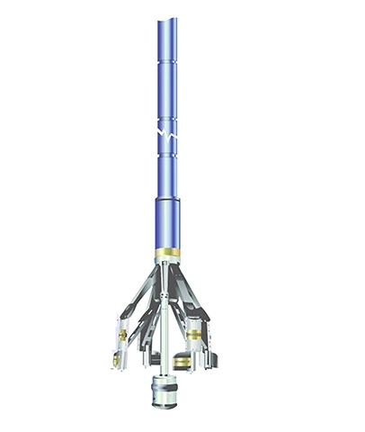
Schlumberger’s acoustical imaging tool (UBI) is shown in Figure 9A.

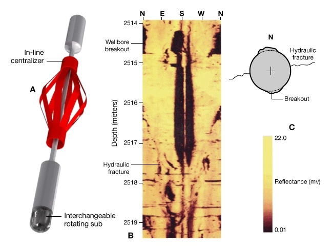
Figure 9B shows a reflected amplitude image of a section of well with both a hydraulically induced fracture and incipient wellbore breakouts. Figure 9C shows the stress direction interpreted for this interval. Notice that the hydraulic fracture and the breakouts are oriented 90 degrees from each other as predicted by the Kirsch equations. The prominent dark vertical band in the center of image is caused by drill pipe rubbing on the wellbore.

Electrical Tools

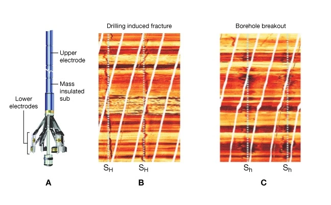
Electrical imaging was invented by Schlumberger in the early 1980s (Ekstrom et al., 1986). Electrical images are formed by an array of electrodes in electrical contact with the formation. Electrode arrays are mounted on multiple mechanically-actuated arms to maximize image coverage of the borehole surface (Figure 10A). Electrical images represent a micro-resistivity map of the rock formation. High resistivity is represented in images as light colors and low resistivity by dark ones. Electrical images provide high-resolution information about fractures and sedimentary structures, but these details often obscure the stress-induced breakouts.

electrical-imaging-tool-FMI — **Figure 10**: A) Schlumberger’s electrical imaging tool (FMI); B) image in a horizontally bedded sequence showing drilling-induced hydraulic fractures; C) image in a horizontally bedded sequence showing stress-induced wellbore breakout

Logging while Drilling (LWD) Tools

A variety of borehole images are also available from logging while drilling (LWD) tools. They include density, resistivity, gamma ray, and ultrasonic images. LWD images may be viewed in real-time and/or recorded in tool memory. LWD images can potentially be used to construct or update a geomechanical model while drilling exploration wells. Real-time imaging is particularly useful for wellbore stability analysis and control.

Stress Direction from Borehole Deformation

Stress direction is one of the most well-constrained components of the in-situ stress tensor. It is determined by measuring the orientation of wellbore failure using oriented multi-arm calipers and borehole images (Figure 5). Impression packers may be used for this purpose but they are not practical or cost effective in most oilfield operations. The majority of stress direction data are obtained from borehole calipers and borehole images. However the azimuth of the fast shear wave has recently emerged as a method for determining stress direction.

Stress Direction from Borehole Calipers

A breakthrough in measuring stress direction in the earth occurred in Canada in 1970 when John Cox, a dipmeter specialist working in the Alberta foothills, noticed that wellbores were preferentially elongated parallel to the mountain front. Almost a decade after Cox’s observations, Sebastian Bell and Ian Gough suggested that the elongation was caused by compressive failure of the wellbore surface (Bell and Gough, 1979). This type of failure was called wellbore breakout and was subsequently confirmed (Figure 5). A competing interpretation of Cox’s data held that borehole elongating resulted from the well intersecting natural fractures (Babcock, 1978), but this hypothesis was not confirmed.

Dipmeter

The dipmeter is a pad-type resistivity tool designed to measure formation dip (Figure 11).

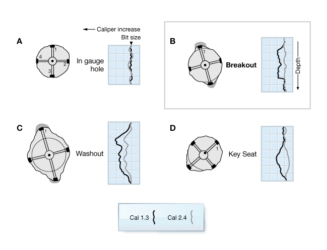
The tool measures micro-resistivity at each of four pads, the azimuth of pad #1, and the borehole diameter in two orthogonal directions. The diameter of the hole between pads 1 and 3 is measured by caliper C1-3 and similarly, the orthogonal diameter is measured by caliper C2-4. Because of the tool design and its deployment on a wireline, the dipmeter rotates as it is brought uphole. When the wellbore is circular, the tool rotates freely; when it is non-circular, one of the caliper pairs becomes aligned with the long axis of the cross-section. The magnitude of the elongation is measured by the calipers. The orientation of the long axis is obtained directly from the azimuth of pad 1, if C1-3 is the long axis, or it is pad 1 azimuth + 90 degrees when the long axis is measured by C2-4.

Figure 12 illustrates the borehole cross-section shape interpreted from dipmeter caliper data. Notice that elongation does not necessarily indicate symmetric damage of the wellbore surfaces as is required for a stress direction interpretation.

Scientific proof supporting the Bell and Gough hypothesis was obtained from a well drilled at Auburn New York (Plumb and Hickman, 1985). Data collected in this well demonstrated that:

Borehole elongation recorded by the 4-arm dipmeter was systematically aligned with wellbore breakout and not natural fractures.
Wellbore breakout was aligned with the azimuth of the least horizontal principal stress.

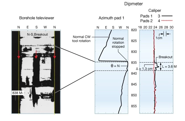
Figure 13 shows a comparison of wellbore breakouts imaged by a BHTV and interpreted from a four-arm dipmeter. Notice that the image reveals damage at diametrically opposed positions on the wellbore surface.

Wellbore-breakouts-shown-by-BHTV-and-dipmeter — **Figure 13**: Wellbore breakouts shown by a BHTV and a dipmeter

Stress Direction from Borehole Images

Borehole images as seen in Figure 10 and Figure 11 can be used to map the depth location and orientation of wellbore breakouts. When the vertical stress is a principal stress and the well is vertical, the azimuth of wellbore breakouts is a measure of the least horizontal stress direction.

As shown previously in Figure 5, hydraulic fractures induced while drilling or created during a stress measurement provide an independent measurement of the maximum horizontal stress direction. The hydraulic fracture imaged in Figure 10 was created during an open-hole stress test conducted in an interval containing wellbore breakouts. Figure 10 C shows that the two structures give an internally consistent orientation for the principal stress axes at that depth location.

Caution is required when interpreting images and calipers from deviated wellbores. Even when the vertical stress is a principal stress, the circumferential position of the maximum and minimum hoop stress concentrations are often not located at the azimuth of the far-field principal stresses. Mastin (1985) describes how borehole deviation and stress regime influences the interpretation of stress direction in deviated wells. A similar caution applies if the vertical stress is not a principal stress. In general, numerical modeling is required to interpret stress from image and caliper data acquired in deviated boreholes.

Stress Direction from Shear Wave Anisotropy

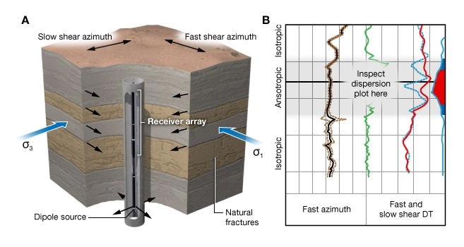
The azimuth of fast shear wave velocity is a reliable measure of the direction of SH when the anisotropy is stress-induced (Figure 14 A). Note that the fast shear azimuth refers to the far-field direction. The existence of fast and slow shear waves is an indication of elastic anisotropy but not whether it is stress-induced. Figure 14 B shows a log of fast shear azimuth in an interval where significant shear wave anisotropy is observed. In this example, the fast shear direction may correspond to the fracture orientation or the direction of $S_H$ . A dispersion analysis can help determine whether the anisotropy is stress-induced or if it is caused by intrinsic rock anisotropy, such as natural fractures or bedding planes.

Dispersion Plot Analysis

A dispersion plot analysis is a requirement for a definitive stress direction interpretation of shear wave anisotropy. Dispersion curves show how shear velocity varies with radial distance from the wellbore, and can indicate whether or not a stress concentration exits near the wellbore (Figure 15). Since flexural waves are dispersive, high frequency components of the shear wave respond to elastic properties within the region affected by wellbore stress concentrations. The low frequency components are governed by elastic properties outside of any stress concentration. Parallel dispersion curves signify intrinsic anisotropy. Crossing dispersion curves signify stress-induced anisotropy.

Shear Velocity Variations Using Dispersion Curves

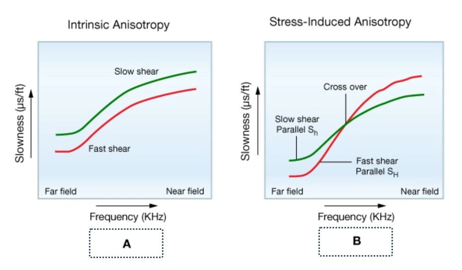
A: This dispersion plot was recorded by a dipole sonic tool for the case of intrinsic anisotropy (for example, due to fractures). Absent a wellbore stress concentration, the fast shear azimuth is constant with radial distance from the wellbore. The dispersion curves for fast and slow shear waves are parallel.

B: When a wellbore stress concentration exists, the low frequency (far-field) components of the fast shear propagate in the direction of SH, but the high frequency components are slowest near the wellbore. Similarly, the slow shear is slowest in the far-field and fastest near the wellbore surface; thus the cross-over seen in in this plot.

In-Situ Stress Measurement

This section discusses borehole measurement of principal stress magnitudes and pore pressure:

Derivation of the Hubbert and Willis breakdown equation
The hydraulic fracturing method for measuring stresses
Pore pressure measurement

The Breakdown Equation

Hydraulic fracturing is the primary method of measuring stress in boreholes due to the Hubbert and Willis breakdown equation (Kehle, 1964; Haimson and Fairhurst, 1967). Building upon the work of Miles and Topping (1949), Hubbert and Willis predicted that fractures induced hydraulically inside a borehole would:

Propagate in a vertical plane perpendicular to the least principal stress, $S_h$ , and
Initiate at the wellbore wall at the azimuth of $S_H$ when the hoop stress, $\sigma _ {\theta}$ , equals the rock tensile strength:

$\sigma\, _{\theta} = - T$

Referring to the hoop stress concentration corresponding to the azimuth of $S_H$ , $\theta$ = 0 (Figure 5):

$\sigma _{\theta = 0} = 3\, S_h - S_H - P_w + T = 0$

and identifying the well pressure, $P_w$ , at fracture initiation as the breakdown pressure, $P_w = P_b$ leads to the classic breakdown equation:

$P_b = 3\, S_h - S_H + T$

Various refinements to the classic breakdown equation have been made to account for pore pressure, the presence of natural fracture, and infiltration of fluids into the rock during a test. However, the form of the breakdown equation given here illustrates the basic stress measurement concept.

Hydraulic Fracturing Stress Measurement

Hydraulic fracturing stress measurements are the primary source of stress magnitude data in sedimentary basins. Note that hydraulic fracturing measures total stress, not effective stress. Conventional hydraulic fracturing stress measurements are conducted in either uncased (open-hole) wellbores using a packer assembly deployed on drill pipe or cased-hole measurements which are gathered through perforations in the casing (Figure 16).

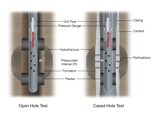
Hydraulic-fracturing-open-hole-vs-cased-hole-test — **Figure 16**: Hydraulic fracturing in an open hole vs. cased hole test

Open-hole Stress Measurement

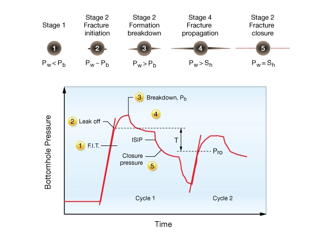
A typical open-hole stress test is conducted as follows.

Identify formations where stress is to be determined.
Identify intervals without pre-existing fractures or planes of weakness.
Set a straddle packer assembly in the target interval.
Using surface pumps, pressurize the interval, until formation breakdown occurs.
Continue pumping to extend the fracture away from the wellbore.
Stop pumping and isolate the interval between the packers from the rest of the hydraulic system and measure the instantaneous shut-in-pressure, $P_w = ISIP$ .
Monitor test interval pressure in permeable formations for a few minutes to identify the fracture closure pressure, $Pw = P_{cl}$ .
Conduct a fracture reopening cycle to measure the formation tensile strength and to check the $ ISIP $ and closure pressures.

In Figure 17, numbers correspond to the wellbore sketches of fracture propagation to the pressure-time record. Drilling terms F.I.T (formation integrity test) and leak off pressure are shown for reference.

Open-hole-stress-measurements-over-time — **Figure 17**: Open hole stress measurements over time

Information from the pressure-time record from a stress test yields the following equation:

$S_h = P_{cl}$

$S_H = 3\, S_h - P_b + T$

$T_0 =P_b - P_{ro}$

The magnitude of $S_h$ and the direction of $S_H$ are the two most reliable quantities obtained from an open-hole stress measurement. The magnitude of $S_H$ is less certain because the breakdown equation does not account for borehole stress perturbations due to natural fractures, irregular borehole shape or fluid invasion into the rock. Consequently the computed magnitude of $S_H$ is likely to overestimate the actual value. However, it is likely that the theoretical breakdown pressure will be greater than what is actually measured. Hence, $S_H$ computed from actual breakdown pressures may be systematically over estimated.

In open-hole tests, the azimuth of $S_H$ can be determined when the induced fracture can be detected and oriented. Originally, hydraulic fracture orientation was obtained using impression packers. Now, borehole imaging is more common. Field studies describing in-situ stress measurements can be found in Hickman et al. (1985) and Evans et al. (1989).

Cased-hole Stress Measurement

Cased-hole stress measurements are more common in the oil industry due to the lower risk of getting tools stuck in the well (Figure 17). A good description of cased-hole stress measurements can be found in Warpinski (1984), and Whitehead et al. (1988). The breakdown equation does not predict fracture initiation from a perforated cased wellbore so cased-hole tests only provide the magnitude of $S_h$ .

Pore Pressure Measurement

Pore pressure is a major component of the total horizontal stress and is required to compute effective stress. It can be measured in permeable formations using wireline or LWD tools. In impermeable formations, pore pressure must be estimated or modeled from geophysical logs.

Pore pressure is typically measured using a fluid sampling tool called a formation tester or similar tool. This is a pad-type device deployed on a wireline (Figure 18B). Pore pressure is interpreted from the pretest pressure record acquired prior to taking a fluid sample. During a pretest, the tool pumps a small volume of fluid from the formation in one or more steps. If the packer seal is good, the pressure measured by the tool builds up to the formation pore pressure. If the seal is bad, the tool measures the well pressure (Figure 18 A).

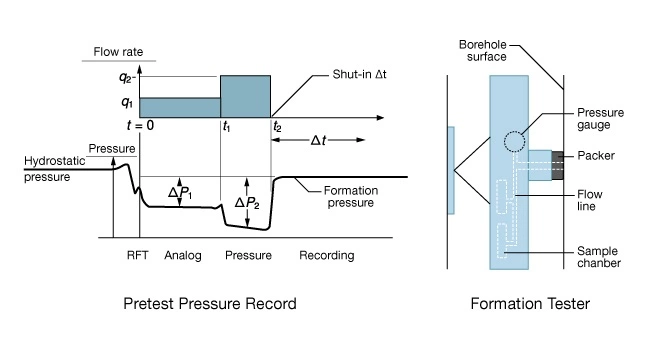
Pore-pressure-measurements — **Figure 18**: Pore pressure measurements

The basic measurement technique is to:

Lower the tool to a permeable zone of interest.
Measure the hydrostatic pressure in the well before setting the packer.
Press the packer into contact with the wellbore surface.
Conduct the pretest.
Interpret pore pressure from the pretest pressure vs. time record.

Recent developments allow hydraulic fracturing stress measurements and pore pressure measurements to be made using a single wireline tool and formation pressure to be measured with LWD tools. LWD technology provides the opportunity to calibrate pre-drill pore pressure and earth models while drilling an exploration well. The wireline technology makes it easier to construct and calibrate more detailed earth stress models in the reservoir.