Interpretation with Seismic Attributes

12 minutes read

Maps obtained for attribute R∗0 PR rotated 45° for the horizons of sands

2D and 3D AVO Attributes

AVO analyzes changes in the amplitude of seismic waves that are dependent on source-receiver distance, and relates to pre-stack seismic attributes for hydrocarbon discrimination. It is an attribute capable of distinguishing if a bright spot is generated by the presence of fluid or just lithological changes.

Figure 1 illustrates the concept of the AVO attribute. In fact, near and far offset-stacks show noticeable differences.

Near and far offset-stacks; arrow A is the reflector of interest, Interpretation with Seismic Attributes, Seismic Attributes, Seismic. geophysics — **Figure 1**: Near and far offset-stacks; arrow A is the reflector of interest

AVO analysis is based on the Zoeppritz (1919) equations. These equations define a relationship between the amplitude of reflection of a seismic wave and the angle of incidence. The change will depend on the density and velocity contrasts (compressional and shear) of the two contacting layers. In fact, in the case of normal incidence, the amplitude of the incident layer is equal to the amplitude of the reflected layer, which depends basically on the densities and velocities of the two media (as shown by the equation below). This is called the P-wave reflection coefficient for normal incidence (NI):

$\dfrac{\rho _2 \, V _{\textrm{p2}} - \rho _1 \, V _{\textrm{p1}}}{\rho _2 \, V _{\textrm{p2}} + \rho _1 \, V _{\textrm{p1}}}$

These relationships become much more complicated when the angle of incidence is oblique. Fortunately, several approximations have been defined in the literature for Zoeppritz equations to allow for a practical application. Shuey’s (1985) approximation is one of the most popular, as defined by Castagna (1994). The P-wave reflection coefficient, as a function of angle of incidence, R_pp(θ), may be expressed as:

$R_{\textrm{pp}}(\theta) = A + B\, \sin^2 \theta$

Where:

A is the normal incidence P-wave reflection coefficient, R_p

B or AVO gradient (or slope) is given by:

$B = -2\, \dfrac{V^2_\textrm{S}}{V^2_\textrm{P}}\dfrac{\Delta \rho}{\rho} + \dfrac{1}{2}\dfrac{\Delta V_\textrm{P}}{V_\textrm{P}} - 4\, \dfrac{V^2_\textrm{S}}{V^2_\textrm{P}}\dfrac{\Delta V_\textrm{S}}{V_\textrm{S}}$

Where:

$V_{\textrm{P}} = \frac{V_{\textrm{P2}} + V_{\textrm{P1}}}{2}$

$V_{\textrm{S}} = \frac{V_{\textrm{S2}} + V_{\textrm{S1}}}{2}$

$\boldsymbol{\rho} = \frac{\boldsymbol{\rho} _2 + \boldsymbol{\rho} _1}{2}$

$\Delta V _{\textrm{P}} = V_{\textrm{P2}} - V_{\textrm{P1}}$

$\Delta V _{\textrm{S}} = V_{\textrm{S2}} - V_{\textrm{S1}}$

$\Delta \boldsymbol{\rho} = \boldsymbol{\rho}_2 - \boldsymbol{\rho}_1$

V_P2= P-wave velocity in underlying medium

V_P1= P-wave velocity in overlying medium

V_S2= S-wave velocity in underlying medium

V_S1= S-wave velocity in overlying medium

ρ₁= density in underlying medium

ρ₂= density in overlying medium

Different authors have proposed different attributes to discriminate gas sands from water-bearing sands. Each of these have advantages and disadvantages. A gas-bearing sand with low impedance laying between shales will show larger negative A and B variables than reflectors that don’t have any associated gas. So the product A×B is a good indicator of gas-bearing sands. Among other indicators, Castagna and Smith (1993) have shown that the indicator R_p−R_s (the difference of the normal incidence P-wave and S-wave reflection coefficient) can work better with gas sands with all kinds of impedances.

Verm and Hilterman (1995) made a different modification of the Shuey’s equation:

$RC(\theta ) \approx NI\, \cos^2(\theta) + PR \, \sin^2 (\theta )$

Where:

NI stands for Normal Incidence reflectivity, as defined earlier

PR= Poisson Reflectivity = $\frac{\boldsymbol{\sigma} _2 - \boldsymbol{\sigma} _1}{(1 - \boldsymbol{\sigma} _{\textrm{avg}})^2}$

Rutherford and Williams (1989) developed a classification for gas-bearing sands based on AVO parameters, which was augmented by Castagna and Swan (1997). Figure 2 illustrates the differences between the four kinds of gas-bearing sands.

Gas-bearing Sands Classifications

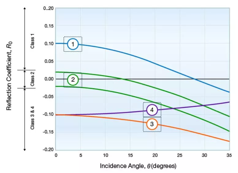
Classifications for gas-bearing sands, Interpretation with Seismic Attributes, Seismic Attributes, Seismic. geophysics — **Figure 2**: Classifications for gas-bearing sands

Class 1: Sands with a greater impedance than the surrounding media where a dim spot is present. The top curve in Figure 2 is representative of a Class 1 sand, which is usually found onshore, is mature and has undergone moderate to high compaction.

Class 2: Sands with a similar impedance as the surrounding media where a phase reversal is present. The middle two curves in Figure 2 represent a range of possible AVO responses in Class 2 sands.

Class 3: Sands with a lower impedance than the surrounding media where a bright spot is present. These sands are usually undercompacted and unconsolidated.

Class 4: The shear velocity (V_s) is less than the V_s from the overlying primarily shale intervals. The sandstone V_s is less than the V_s of the shale interval above it.

Castagna and Swan note that Class 3 and 4 gas sands may have identical normal incidence reflection coefficients, but the magnitude of Class 4 sand reflection coefficients decreases with an increasing angle of incidence, while Class 3 reflection coefficient magnitudes increase.

Plots of A versus B (or the gradient versus R₀) allows for discrimination of gas-bearing sands from water-bearing sands or dry sands.