Seismic Interpretation Methods

Learning Objectives

After completing this topic ” Seismic Interpretation Methods “, you will be able to:

• Explain the purpose of seismic modeling and how it aids seismic interpretation.
• Describe how the amplitude, polarity, and shape of the seismic signal are important to understanding the geological lateral variations of the subsurface.
• Differentiate between bright spots, flat spots and dim spots on seismic sections, and explain what causes these direct hydrocarbon indicators.
• Discuss and identify the three reflectivity zones according to their individual characteristics.
• Outline how crosswell seismology provides high density, depth-calibrated seismic data between two wellbores.

Seismic interpretation is the process of analyzing seismic data to understand the geology and structure of the subsurface. It is an essential step in the exploration and production of hydrocarbon reserves. The process of seismic interpretation involves the use of various methods and techniques that help to extract geological information from the seismic data. In this article, we will discuss some of the most commonly used seismic interpretation methods.

Seismic Modeling Introduction

Seismic modeling is a very useful way of testing the validity of a particular interpretation. Seismic data interpretations are ultimately based on models, which may employ both qualitative concepts and quantitative frameworks. Our focus in this course is on quantitative models that, when used with seismic data, form a basis for exploration decisions and reservoir definitions.

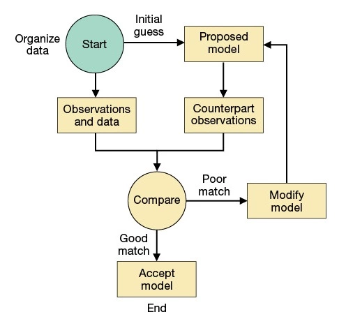
The standard of acceptance for any model is its consistency with the actual data. By using quantitative mechanisms, we can apply quantitative measures of consistency as a means of comparing and prioritizing opportunities. As shown in Figure 1, it is a straightforward matter to organize a logical sequence for testing models, whatever their form.

Geologic parameters as well as seismic can be changed to produce different artificial responses of the Earth model. Animation 1 illustrates the process for constructing a synthetic seismogram.

Building of a synthetic seismogram

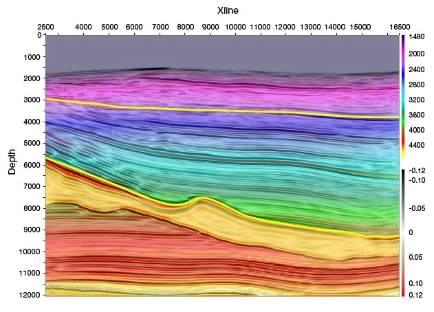
Analysis of the amplitude, polarity, and shape of the seismic signal is an important step in understanding the geological lateral variations, or stratigraphic model, of the subsurface.

Figures 2-4 show an example of the use of seismic modeling to support the interpretation of a complex geological section.

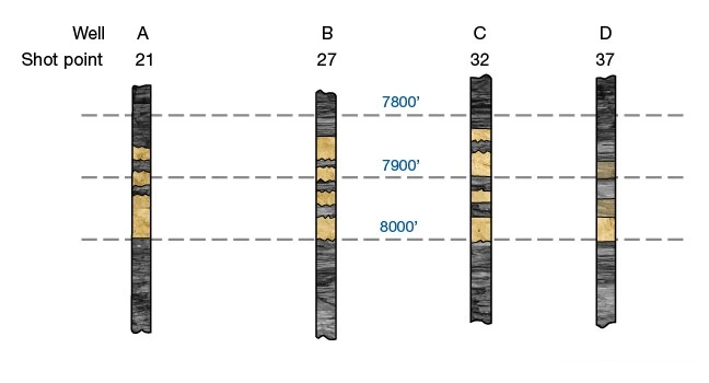
Control for the model is provided by wells A, B, C, and D located at shotpoints 21, 27, 32, and 37, respectively (Figure 2). The stratigraphic columns were derived from each well’s logs and show a basal sand unit with an inter-fingering sand-shale sequence above. The sandstone layers have a uniform and constant velocity that is slower than the surrounding shale.

The proposed input model (Figure 3) illustrates the lateral lithologic transition. The four well locations are also indicated in this figure. Notice the lack of well-defined boundaries this will influence the seismic reflections by producing gradational responses rather than sharp, distinct changes at the boundaries. Also note that there will probably be Fresnel zone effects where the gaps between sand fingers are narrow.

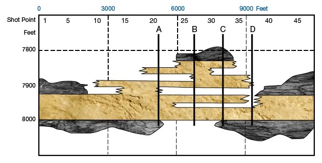
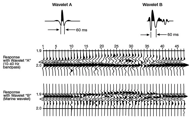
Between shotpoints 24 and 38 the basal sand is thinner due to an interbedded layer of shale. The proximity of this interface to the base of the sandstone causes interference and produces distortion of the total seismic response. The resulting wave theory synthetic seismic sections are shown in Figure 4, where we see two sections using two different wavelets.

The convolving wavelet (A) is a standard 10-40 Hz bandpass wavelet, symmetrical in shape and polarized so that a positive reflection corresponds to a peak on the seismic section. In the corresponding section, we see that the base of the sandstone shows a nearly consistent high-amplitude peak and arrival time. The only variations in amplitude or time occur between shotpoints 24 and 34, where the sandstone layers are collectively the thickest. In this interval, the basal sand reflection becomes less consistent in waveform, decreases in amplitude, and increases somewhat in traveltime, producing a small sag in the reflecting horizon. We would expect this sag in time because the average velocity within this interval is slower than in the rest of the model due to the greater thickness of low-velocity sand within this interval. The waveform distortion and loss of amplitude, however, are due not to the greater sand thickness within this interval, but to interference.

Above the basal sand reflection in Figure 4 (wavelet A), we note very little continuity in the seismic response. The only continuous reflection that we see is a negative low-amplitude event that defines the top of the sandstone envelope. We note that the trough arrives earliest in the section where the sandstone is shallowest in the model. Beyond the lateral limits of the highest sand fingers, both to the right and to the left, we note the increase in amplitude of the trough, which indicates the absence of shallow sands. However, between shotpoints 10 and 40 and above the basal peak, we see no correlation between the synthetic seismic section and the input model. Thus, when the boundaries between layers are diffuse, the seismic response is not as indicative of the geologic model.

To summarize this particular model, if we are looking for the location where the sands are best developed we look for:

1. The loss of the trough to define the lateral boundaries of sand development
2. The trough to arrive earliest where the sands are the shallowest
3. A time sag in the basal sand reflection to indicate where the sands are thickest

Now we’ll examine what happens if we use a typical marine airgun wavelet (B), one that is neither symmetrical nor regular, to produce the synthetic section.

We immediately notice a dramatic difference in the appearance of the seismic section generated by the marine wavelet (B), compared to the one we generated using the standard wavelet (A). The most striking difference is the change in the basal sand reflection. In the first section, we saw a strong positive reflection, but in second section we now see a weak doublet. The base of the sandstone would now possibly be more difficult to recognize if a high level of noise were present. We also no longer see the time sag we saw in the previous section, nor do we see any change in the doublet waveform across the section. Notice, however, that the strong trough now becomes more continuous across the entire section, although it does lose some of its amplitude where the sands are thickest. The greatest interpretational gain from this wavelet is the better definition of the upper sand interfaces. We can more clearly see the stair-step appearance of the uppermost reflection, indicative of the sand fingers building to a high between shotpoints 24 and 34 and decreasing on either side.

This exercise reinforces the importance of selecting an accurate wavelet. We cannot readily determine which wavelet to use just by comparing the two resulting synthetic sections. The only way we can determine the correct wavelet is to compare the modeled results to the recorded and processed seismic data. If the synthetic traces match the real seismic data at the control points, then we know the wavelet used is a good choice. If the two do not match, then we need to define a new wavelet.

Seismic modeling is explored with much greater detail in the Seismic Stratigraphic Modeling topic, and in the Seismic Modeling course in the Hydrocarbon Indicators topic.