Geosteering Practices

Geosteering Interpretation Techniques

Several interpretive methods are currently used within the industry for geosteering. Some work better than others, but none are universally successful -and all methods have their own disadvantages.

Geometric Steering

Geometric steering is a method in which all “geosteering” is performed before the well is drilled. This means that a plan is developed based upon the best geologic data available, and then the well is drilled with no re-evaluation of the geology while drilling. Steering is based only on bit direction and inclination data.

Any gamma ray and resistivity (or other) logging data will probably be measured far behind the bit, and will be used only after the section has been penetrated.

Data Requirements:	Pre-drill model, no additional data used.
Application:	This method can be used in thick targets with fairly homogeneous stratigraphy and predictable structural architecture. It is often used when drilling above a water contact.
Pitfalls:	There are few reservoirs with homogeneous stratigraphy and predictable structural architecture that are drilled with horizontal wells. It is less effective when the target is thin, structurally complex, or insufficiently mapped for planning well trajectory. Geology is never as simple as we believe. Without data, there is no way to evaluate the accuracy of the placement of the well in the stratigraphy.

It is important to examine other data to ensure that the well stays above any water contacts because of wellbore position uncertainty.

Marker Bed Search Method

This method uses obvious stratigraphic markers to “bracket” the target. When the well drills out of target it is determined whether the well has drilled out the top or bottom by determining which “bracket” marker has been penetrated. Average dip rates are calculated between marker penetrations. When a well faults out of target, the geologist must make the best guess of the direction to the target.

Data Requirements:	Sample descriptions and gamma ray amplitude to determine whether a well is in or out of zone.
Application:	This method can be used where the target is distinct and where the beds below and above the target exhibit a significant difference in gamma amplitude.
Pitfalls:	This method is risky where the stratigraphic sequence is cyclical; if a fault is cut and the well is thrown from one similar sequence to another, it will never be known. If the well is faulted beyond the bracketing beds, the geoscientist has a 50% chance of steering the well back into target on the first try. Tagging markers to obtain average dip rates puts unnecessary doglegs in the well that can jeopardize the wellbore.

Visual Correlation of Horizontal LWD Logs

This method consists of correlating either the measured depth LWD logs or TVD logs manually with vertical offsets. However, both measured depth LWD logs and TVD logs will be severely distorted because of the interaction of wellbore geometry and the geology through which the well is drilling. This distortion is predictable through the build section, and can be easily accounted for, but the distortion becomes more complex during the lateral section.

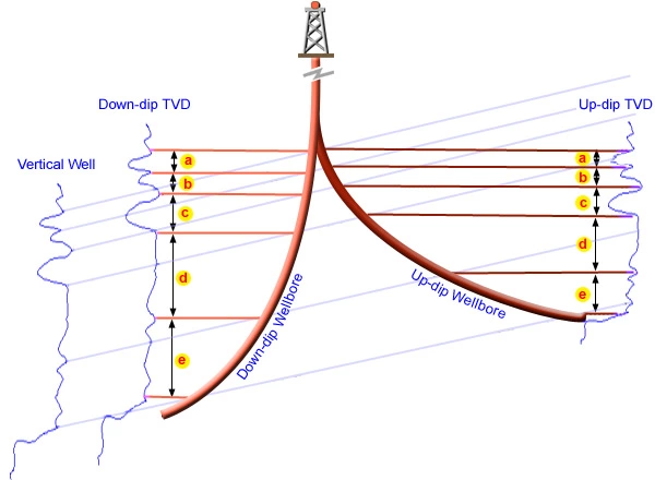
The TVD log can be used through the build section to correlate with logs from offset wells as long as it is recognized that the TVD log will be thinner in a horizontal well that is drilled up-dip and thicker in a horizontal well drilled down-dip (Figure 1: Well log distortion).

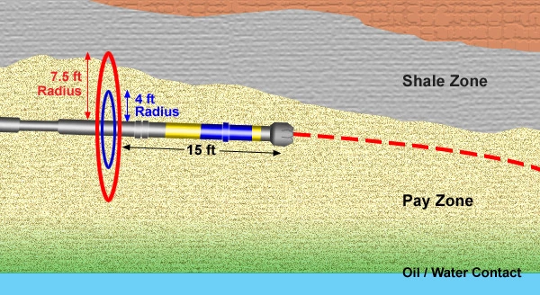
Because of this phenomenon, the height above target must be calculated by using the thickness from the offset vertical well between the last correlation point and the top of the target. In measured-depth, the amount of formation exposed will vary according to the wellbore geometry: Up-dip/Up-section wells will expose more of a formation than Up-dip/Down-section wells. Similarly, Down-dip/Down-section wells will expose more formation than Down-dip/Up-section wells (Figure 2).

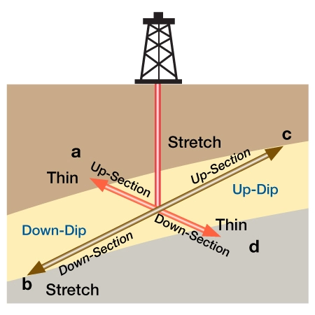
In this figure, we see that wellbore a is much shorter than wellbore b, and that wellbore cis shorter than wellbore d. Such shortening or lengthening of formations can wreak havoc on the correlation process.

Measured depth logs can be reduced by optical shrinking in order to attempt to correlate with offset wells, but this becomes difficult (if not impossible) when the well is in the lateral section. There is generally just too much interaction between the wellbore geometry and the formation to do this manually.

It is also important to consider the SCALE of the logging data used in the correlation process. Figure 3 compares gamma ray data presented on two different scales.

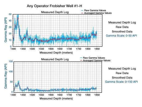
The correct scale to use will always depend on what you want to look for, but will typically be the scale that provides the easiest correlation with the offset logs.

Data Requirements:	LWD correlation log -such as gamma ray in the build section.
Application:	Correlate through the build section.
Pitfalls:	Distortion of the log in the horizontal section of the well makes this correlation very difficult and often impossible in the lateral section. Once a well is near 90 degrees, the TVD log is quite useless.

Forward Modeling of Measured Depth Resistivity LWD Logs

This method is utilized by all of the directional contractors that have a geonavigation interpretation method, including Schlumberger/ Anadrill, Halliburton/ Sperry Sun, Pathfinder, and Baker Hughes/Inteq. The method utilizes an extensive pre-drill model, typically developed on the basis of well control, with additional input from seismic data. Based upon the pre-drill model, a grid of interpolated resistivity logs is created. The modeled vertical logs are then stretched, based upon the proposed wellbore geometry and pre-drill structural model. This creates a pre-drill modeled resistivity log that can be correlated against the measured depth LWD log. As the well is drilling, the system re-stretches the model log based upon the new surveys and the pre-drill structural model. If the re-stretching does not cause the curves to overlay the pre-drill structural model is changed until the modeled log and the LWD curves overlay.

The method works well when the pre-drill model has enough data control to be very accurate, and when there is very little faulting in the area. (Unexpected faulting or faults below the resolution of seismic will complicate the modeling process.) After cutting a fault (even a tiny fault), it is important to determine the new stratigraphy into which the well is thrown. Since this method correlates on a measured-depth reference rather than a stratigraphic reference, it can be very difficult to pick the new location across a fault.

This method uses the wellbore as the reference for all calculations. This system was primarily developed to accommodate an engineering perspective, with all data referenced to the wellbore. It is used by a number of directional contractors.

The problem with using measured depth as a reference is that measured depth has no stratigraphic significance. As a result, it is difficult to pick faults with this method, and is even more difficult to place the well within the pay section after encountering a fault.

As mentioned in earlier, resistivity is not always the best tool to use for correlation since the resistivity in a reservoir can change rapidly in a reservoir with lateral changes in porosity and water saturation. The method, however, can be used quite effectively in areas where an oil / water contact must be avoided. The approaching water contacts can often be detected quite well with this method by watching the gamma and the resistivity correlation. If the gamma values appear to remain in target while the resistivity begins to drop, then it is probably time to alter course and steer away from the oil / water contact (Figure 4).

The method can also incorporate other curves for correlation.

Data Requirements:	LWD resistivity and gamma ray. Optional logs are density, neutron, and sonic. Also need Directional surveys and an accurate, pre-drill structural model that is based on offset wells.
Application:	Steering in areas with fairly predictable geology, or when trying to stay away from a water contact.
Pitfalls:	The method requires correlation of measured depth logs that still have not been compensated for the distortion caused by directional drilling. Resistivity is great for seeing beds and oil / water contacts away from the wellbore, but is not the best correlation tool. The method uses measured depth as the correlation reference rather than the stratigraphy. Identifying faults not seen in the pre-drill model can be problematic

Biosteering

Biosteering provides yet another interdisciplinary approach to geosteering, tying together aspects of production geology, biostratigraphy, and drilling. Adopted by BP, the company has used biosteering in over 200 wells in 20 fields worldwide since 1995. Given enough paleontological data, biosteering provides reservoir-scale stratigraphic control that can help the Geosteering Team ascertain where a high-angle or horizontal well is within the stratigraphic column, and is becoming an important part of the geosteering toolkit.

Pre-drill planning involves detailed studies of the reservoir to characterize the biostratigraphy of the field. The process begins by delineating unique stratigraphic layers to subdivide the reservoir into correlatable time-slices. Each individual layer is defined by certain field-specific microfossil bioevents. By layering the reservoir at a higher resolution than regional, exploration-scale biostratigraphy, this approach often provides greater resolution than seismic while covering a greater area than well logs. Thus the biosteering pre-drill phase helps the geologist to better understand the extent of heterogeneity within the reservoir, and helps to show which parts of the reservoir may be connected.

At the wellsite, biosteering requires diligent attention to sample collection. Formation cuttings are collected at the shale shaker, and then prepared and analyzed by a wellsite paleontologist. This process usually takes less than two hours, which means that measurements and interpretation may made in timely fashion, but do not take place in real-time (i.e., if ROP is 10 m / hour, then the biostratigraphic interpretation will be at least 20 meters behind the bit).

In clastic reservoirs, the fossil-bearing intervals consist of muds and silts that envelop and subdivide the pay. In carbonate reservoirs, the entire interval will probably be fossiliferous. By recognizing and correlating defining bioevents from the rig, the paleontologist can help the Geosteering Team determine the stratigraphic position of non-pay units, such as mudstones or siltstones. Above the target pay zone, biostratigraphy is used in an ongoing comparison with offset well data to determine whether horizons are coming in deeper or shallower than anticipated. With this information, the Geosteering Team can adjust well trajectory to land within the target zone between the non-pay intervals. Biosteering is particularly useful when a well intercepts an unanticipated, sub-seismic fault. The Geosteering Team will then rely on the paleontologist to determine whether the well has crossed above or below the pay zone, and then guide the well back to the pay interval.

Biosteering has been applied to shallow-or deep-marine clastic or carbonate reservoirs, and shows great potential across a broad range of geo-provinces, including the deepwater Gulf of Mexico, Angola, Azerbaijan, Egypt and Trinidad.

Data Requirements:	Formation cuttings, collected at the shale-shaker, and biostratigraphic data from offset wells.
Application:	Excellent correlation through the build section, particularly useful for determining position after cutting faults.
Pitfalls:	Recalling the earlier discussion on problems with formation cuttings, this method depends on samples that must first be circulated up from TD, and which may not reflect the true position of the bit, due to contamination from other zones, or due to lost circulation. The circulation process and sample preparation time means that stratigraphic position cannot be determined immediately upon cutting the formation. Furthermore, this process depends on correlations with offset wells. If paleontological samples were not obtained from nearby wells, then this method will not be able to achieve the degree of resolution needed for making crucial geosteering decisions.

Seismic Steering

Seismic data can serve as a useful tool for steering a well, but should not be solely relied upon without input from LWD interpretation. The basic problem with using seismic as a sole source for geonavigation stems from the fact that seismic is recorded in the time domain, while wells are drilled in the depth domain. A time-to-depth conversion must be performed on the seismic to transpose it to the correct depth domain. The time-to-depth conversion requires an interpretation of velocity relationships, which has the potential for adding error to the conversion. Without an accurate time-to-depth conversion, seismic data can only be used as a subjective guide in horizontal navigation. This is true regardless of the quality of the seismic.

Techniques for tying in vertical wells to seismic are well established, even when a velocity survey has not been run in the well. A synthetic seismogram can be generated from the vertical log, which is then correlated to the seismic section. Primary seismic markers are identified to tie stratigraphic events with certain reflections on the seismic data. The target may then be defined in reference to these “primary seismic markers”.

Creation of a synthetic seismogram becomes problematic with horizontal logs. A synthetic seismogram of a measured depth horizontal log is quite useless because the measured depth log does not represent a model of the stratigraphic section. Similarly, a TVD log does not factor out distortion caused by wellbore inclination, nor does it correct for formation dip.

The only way a meaningful synthetic seismogram can be made is to know the true stratigraphic position of each point within the well. The data in the vertical portion of a horizontal well can be combined with a TSP log through the curve to tie with the seismic data using a synthetic seismogram. This provides a tie to the seismic at the surface location. Once the stratigraphic position of the lateral section is known, then an accurate interval velocity can be calculated between the wellbore position and a primary seismic marker. Likewise, an average velocity from the surface to some point within the wellbore can be calculated to more accurately portray the seismic in the depth domain. This process can be repeated as often as necessary while the well is drilling. This adds a predictive aspect to geonavigation that LWD logs or seismic alone do not provide.

The great majority of horizontal wells are drilled within or near a two-dimensional plane, so 3D visualization techniques are not always beneficial. However, if the wellbore is planned with a variable azimuth, then 3D visualization becomes more important, and 3D seismic can be especially helpful in these cases. The wellbore can be plotted within the 3D cube to more accurately predict geology in front of the bit.

It is very important to note that most horizontal targets are actually thinner than the seismic data can resolve. Cases where the target is very shallow, the data is of exceptional quality, and where seismic can accurately discern character within the target are NOT the norm. In most cases, the operator can only see a reflector near the target from which structure is interpreted. Again, it is important to stress that most reservoirs have faults which fall below the resolution of the seismic data. Just as the outcrop reveals small faults with throws from less than a foot, to throws of 20 feet or more, such faulting may not be seen at depth on a seismic section, yet they can play a major role in the targeting of a horizontal well.

Data Requirements:	Seismic data (preferably 3-D data volumes) acquired through the area of interest, and in the ideal case, the data would be shot through the well location and along the proposed wellbore path. A velocity survey and/or synthetic seismogram should also be run in order to convert from a time to depth domain.
Application:	Used primarily above the landing zone to tie seismic reflectors with key stratigraphic intervals.
Pitfalls:	Once the well has landed in the target zone and lateral drilling commences, the synthetic seismograms and velocity surveys become useless. Also, seismic usually cannot resolve small faults which can throw a horizontal wellbore out of the target zone.

True Stratigraphic Position Modeling

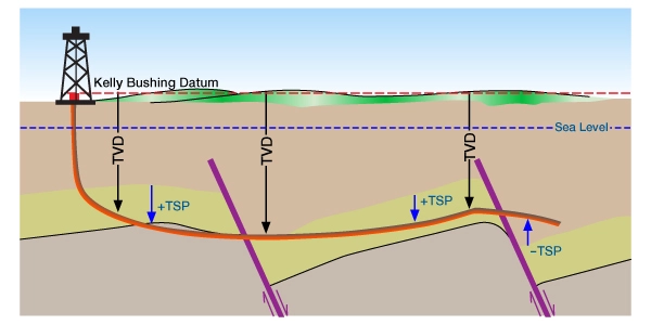
True Stratigraphic Position Modeling (TSPM) is a method used to transpose the LWD data from its position in the wellbore to its position within the vertical stratigraphic section (or True Stratigraphic Position) An example of the problem geometries is shown in Figure 5).

Using this method, the stratigraphic distortions caused by the interaction of wellbore trajectory and formation dip are removed from the measured depth log. The resulting calculated log is called a True Stratigraphic Position (TSP) log, as shown in Figure 6.

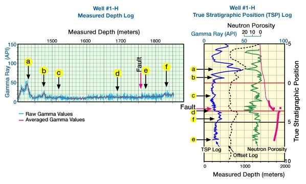
This Figureshows two logs: the left side of the frame shows a measured depth presentation of the LWD gamma ray log, with key points designated a-f on the log, and the right side shows how that gamma ray data is presented in the corresponding TSP log, with corresponding points a-f.

The TSP log display is explained in detail below.

TSPM First Pass

A first-pass TSP log is generated using an average dip or a dip predicted on the basis of the prospect’s structural model.

Next, a correlation is made between the first-pass TSP log and a representation of the stratigraphic section. The representative stratigraphic section has been modeled on the basis of offset well data, or is taken from a previous portion of the horizontal wellbore that has already been successfully modeled.

If the data is not transposed to its proper stratigraphic position, the model must be modified until the observed correlation matches the known stratigraphic section.

The TSPM method corrects the MD log, thus creating a simulated vertical log that can be used to correlate in the same manner as two vertical logs are correlated.

Dynamic Correlations

The TSPM correlation model evolves as the well is drilled, changing to conform to observed data. Faults and gradual facies changes are incorporated into the model as they are readily identified using the TSPM method.

Often, data in a horizontal well may be correlated against the last pass-through section, which may only be feet away. Faults with throws as small as 0.3 meter or 1 foot can be identified because of the detailed stratigraphic information recorded in LWD gamma ray logs and the short distances correlated. Individual fault blocks can be displayed on the TSP log in their correlative position within the stratigraphic section. When available, multiple offset logs should be utilized in the model so that gradual facies changes can be recognized and properly interpreted.

Two Views of the TSPM

The model is displayed in two parts:

• TSP log – represents a restored stratigraphic cross-section between the TSP interpretation from the horizontal wellbore and the offset correlation logs.
• Wellbore Plot – a structural cross-section plotted along the wellbore path.

TSP Log Display

The TSP log represents the stratigraphic correlation that was made through the modeling process. The components of the TSP log include (Figure 7):

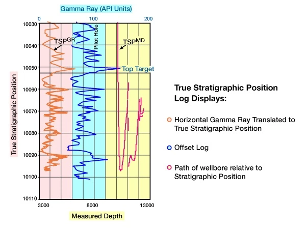
• the calculated TSP gamma ray curve (sometimes a log other than gamma ray may be used), (these curves are presented on the left side of the plot);
• the offset log, usually taken from a nearby vertical well (black log curve in the center of the plot);
• the stratigraphic path of the wellbore, (magenta curve on the right of the plot); and
• a text box detailing the last survey data.

Interpreting the TSP Log Display

Let us take a closer look at a typical TSP Log. Figure 8:

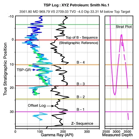
First, we see that the log is annotated with various target zones. These targets are based on the GR curve from an offset well (the black curve posted in the middle of the log).

Next, look at the text posted at the top of the log. We see that the well has reached a measured depth of 3561.8 meters, and is presently 33.31 meters below the Top of Target. This depth is reflected by the magenta curve at the right-hand side of the log.

Let us concentrate on the magenta curve on the right-hand side of the log. This stratigraphic wellbore path (TSP-MD) tracks the progress of the drill through the target section. On this segment of the log, we see that this curve starts at 2750 meters MD (read this measurement against the depths posted along the bottom of the log), and ends at a TD of 3561 meters. This curve also shows that the wellbore undulates from 23 meters below the stratigraphic reference (Top of B Sequence) to 2 meters above the target, before finally dropping back down to 33 meters below the stratigraphic reference (read these depths along the left side of the log).

Faults show up clearly as breaks in the magenta TSP-MD curve. On this log, we can see where the wellbore drilled into a fault just below the B-3 zone, at about 3515 meters (MD), with the result that the B-2 zone was completely faulted out before the well encountered the upper B-1 zone. Also, an 8-meter gap in the correlation provided by the blue TSP-GR (on the left side of the log) corresponds to the fault gap in the magenta TSP-MD curve.

Wellbore undulations cause the TSP-GR curve to re-trace its position. Note that the TSP-GR curve (left-hand side of the log) repeats itself along a corresponding interval for each undulation that the magenta TSP-MD curve makes. (In this display, the TSP-GR curve is split into dark blue, light blue, and light green curves to show successive repetitions.) This re-tracing makes the TSP-GR curve increasingly thicker with each undulation of the TSP-MD curve. This gives the geoscientist a qualitative check of the correlation upon which the model is based.

When compared to the GR curve from the offset well, we see that the LWD GR log presented as the TSP-GR curve exhibits much better stratigraphic resolution than that of the offset well. This offset log is used for correlation until the target stratigraphic section has been penetrated by the wellbore. The model is then based upon the correlation with data in the lateral wellbore that has already been modeled.

TSP Wellbore Plot Display

The Wellbore Plot is a structural cross-section projected to the vertical section plane of the proposed azimuth. This plot is shown in Figure 9.

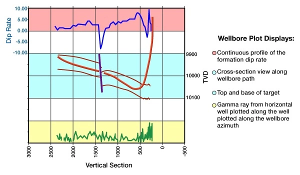
The components of the Wellbore Plot include:

• a plot of the LWD GR data along the vertical section (at bottom),
• the top and base of target and other formation tops (middle plot),
• the trace of the wellbore trajectory (middle plot, where wellbore is shown as heavy black line), and
• a continuous profile of the apparent formation dip.

Interpreting the TSP Wellbore Plot

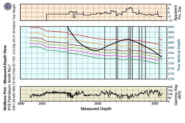
Starting at the bottom of the log, (Figure 10) we see an LWD GR plot, displayed in measured depth. The raw LWD data are plotted along the vertical section, providing a reference to the distance away from the KOP.

The middle plot presents a cross-section that clearly shows the structural position of the wellbore relative to the intended target. In this example, the wellbore undulates through a number of zones.

At the top of the log is the Apparent Dip curve, one of the most useful components of the Wellbore Plot. Knowing the apparent formation dip is critical to staying in the target. This curve allows the operator to stay closer to the bed, drilling parallel with less sliding to correct the trajectory. A continuous formation dip profile also means that the well-site geologist will not have to tag the top of the zone to check the “average dip”.

(The Apparent Dip curve is an interpretive product that is “driven” through a process of iterative correlations between the LWD-GR curve on the TSP log and the offset correlation log. Adjusting the apparent dip angle between correlation points causes the log to stretch or compress in order to match the correlation from the offset log.)

Data Requirements:	Gamma Ray LWD. Optional logs include resistivity, density, neutron, and sonic.
Application:	Geonavigation of most targets where a correlation can be made between vertical offset logs over a distance of half the proposed lateral length. The method works especially well in areas of complex structure.
Pitfalls:	The method is a correlation method that requires extensive interpretation. The method does not work well for wells drilled in braided stream environments, reef core or other environments with chaotic deposition.