Related Articles


Linear Elasticity
The theory of linear elasticity relates stress to strain (such as rock deformation) and strain to stress. Linear elasticity forms the theoretical basis for determining elastic moduli of rocks and for estimating earth stresses. It is consistent to use linear elasticity to describe rock deformation subject to two restrictions:
- Infinitesimal strain approximation applies.
- Rock stresses do exceed the yield stress.
Hooke’s Law
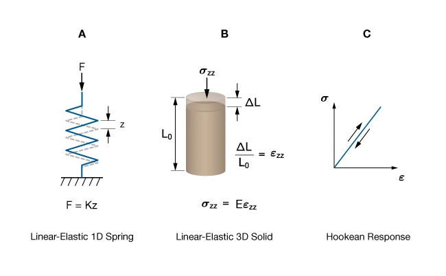
The foundations for linear elasticity were discovered in the 17th century by Robert Hooke who was experimenting with springs. Hooke observed that the elongation of a spring was linearly proportional to the applied force. Hooke’s Law is given by:

Where  is the elongation of a spring due to applied force
  , and
, and  is the spring constant. Imagine that the one-dimensional spring is replaced by a three-dimensional cylindrical specimen of rock. By analogy, the linear deformation of the rock,
  , subjected to an applied stress,
  , can be expressed as:

where  is the modulus of elasticity or Young’s modulus, named after the 19th century British scientist, Thomas Young (Figure 1).
Stiffness Tensor
In order to compute stress from applied strain the components of the stiffness tensor need to be specified. Components of the stiffness tensor are given in units of stress because strain is dimensionless. For the most general anisotropic material, the stiffness tensor has 81 components. Because of symmetry of the stress and strain tensors, the number of independent components reduces to 21 (Nye, 1957). For the special case of isotropic materials, (ones whose elastic properties do not vary with direction) there are only two independent components or elastic parameters.
There are six linear equations relating stress and strain through the stiffness tensor. Geophysicists prefer to work with Lame’s parameters:  and
and  , because these are two material-dependent quantities. The stress and strain relations for an isotropic solid in terms of and are:


Where the coefficient is called Lame’s first parameter and is Lame’s second parameter. is also called the modulus of rigidity or the shear modulus. In principal coordinates the six equations reduce to three:
Petrophysicists find it more natural to work with the Bulk modulus,  and shear modulus,
  . In rock mechanics and geomechanics it is common to work with Young’s modulus
  and Poisson’s ratio
  . Principal stresses expressed in terms of
 ![E[latex] and [latex]\nu[latex] may be written as: <!-- /wp:paragraph --> <!-- wp:paragraph --> [latex]\sigma {xx} = \dfrac{E}{\left ( 1 + \nu \right )\left ( 1 - 2\nu \right )}\left [ \left ( 1 - \nu \right )\varepsilon {xx} + \nu \varepsilon {yy} + \nu \varepsilon {zz} \right ]](https://petroshine.com/wp-content/ql-cache/quicklatex.com-544dbb02d9dc60a3aa1a1ff5d2bbbc5c_l3.png "Rendered by QuickLaTeX.com")
![\sigma {yy} = \dfrac{E}{\left ( 1 + \nu \right )\left ( 1 - 2\nu \right )}\left [ \nu \varepsilon {xx} + \left ( 1 - \nu \right ) \varepsilon {yy} + \nu \varepsilon {zz} \right ]](https://petroshine.com/wp-content/ql-cache/quicklatex.com-5e21fb4d5879545a8c90c66d2e979a6a_l3.png "Rendered by QuickLaTeX.com")
![\sigma {zz} = \dfrac{E}{\left ( 1 + \nu \right )\left ( 1 - 2\nu \right )}\left [\nu \varepsilon {xx} + \nu \varepsilon {yy} + \left ( 1 - \nu \right ) \varepsilon {zz} \right ]](https://petroshine.com/wp-content/ql-cache/quicklatex.com-4943ee3f585525fb59feb7323c138b82_l3.png "Rendered by QuickLaTeX.com")
Note that in-situ stresses obtained by hydraulic fracture stress measurements or by modeling are commonly expressed as principal stresses.
Table 1 shows relationships among the various elastic moduli for isotropic materials in terms of commonly used independent pairs (, ), (,  ), and (,
  ) (Jaeger and Cook 1976).
| Table 1: Useful conversion between elastic parameters | |||
|---|---|---|---|
Compliance Tensor
The compliance tensor relates strains to applied stress. The units of compliance are inverse stress. Most laboratory measurements of rock deformation are reported as principal strains. Strains are measured by instruments that record the rock’s response to loads applied by the testing machine.

Principal strains in terms of and may be written as:
![\varepsilon _{xx} = \dfrac{1}{E} \left[ \sigma _{xx} - \nu \left( \sigma _{yy} + \sigma _{zz} \right) \right]](https://petroshine.com/wp-content/ql-cache/quicklatex.com-b0fadd18294c80f172f16499d66fa4d0_l3.png "Rendered by QuickLaTeX.com")
![\varepsilon _{yy} = \dfrac{1}{E} \left[ \sigma _{yy} - \nu \left( \sigma _{xx} + \sigma _{zz} \right) \right]](https://petroshine.com/wp-content/ql-cache/quicklatex.com-19bbfc1bc39b8e80368f291b2041dce3_l3.png "Rendered by QuickLaTeX.com")
![\varepsilon _{zz} = \dfrac{1}{E} \left[ \sigma _{zz} - \nu \left( \sigma _{xx} + \sigma _{yy} \right) \right]](https://petroshine.com/wp-content/ql-cache/quicklatex.com-ec3dcede4aa15019e30e7e3a25c0094b_l3.png "Rendered by QuickLaTeX.com")
Poroelasticity
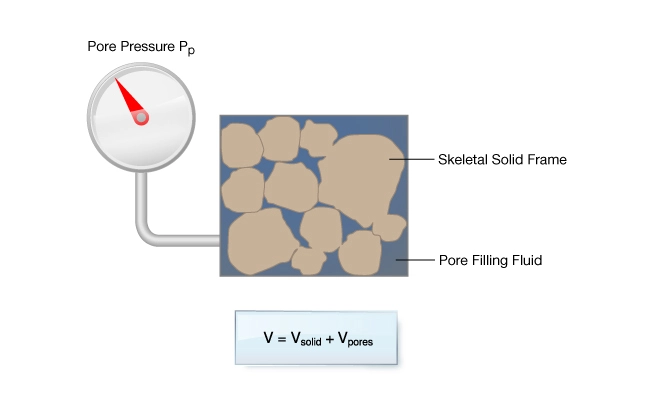
Sedimentary rocks of interest to the petroleum industry are porous fluid-saturated materials. The presence of fluid-filled pore space produces a more complex stress-strain response in poroelastic solids than in elastic solids. The theory of poroelasticity accounts for the contribution of pore fluids to the deformation of the solid. The presence of fluid in a poroelastic material leads to two characteristic behaviors:
- Solid-to-fluid coupling, whereby a change of stress on a porous material either changes the fluid pressure or the mass of fluid
- Fluid-to-solid coupling, whereby a change in fluid pressure or fluid mass induces a change in volume of the porous material
Figure 2 illustrates a fluid-saturated poroelastic solid of volume V comprised of solid volume, Vs, pore volume, Vp, and internal pore pressure Pp.
The first general theory of 3D poroelasticity was published in 1941 by Maurice Biot, a Belgian-American engineer. His theory is based on infinitesimal elasticity theory. Biot showed that for isotropic porous rock, fluid-rock coupling only impacts the volumetric part of the stress-strain relationship.
Biot’s theory is important to geomechanics in the following ways:
- Effective stresses are normal stresses. The generalized expression for the effective stress tensor is:

- Biot’s effective stress contains a term (
 ), multiplying the pore pressure term. represents the efficiency with which pore pressure counteracts externally applied loads. An intuitive micromechanical definition of is given by:


where is the bulk modulus of the rock and  is the bulk modulus of the solid material making up the skeletal frame, for example the mineral grains. Notice that
  approaches 1 when
  .
.
- Rocks may deform under drained or undrained conditions. A drained response is any deformation where fluid volume changes but pore pressure,
 , does not. A drained response is slow enough that there is no induced pore pressure. An undrained response is one where the fluid volume does not change but does. An undrained response is so fast that the fluid cannot flow, thus leading to an increase in pore pressure.
 - Elastic parameters used in poroelastic constitutive relations are “drained” (the so-called frame moduli, indicated by the subscript
 . Specification of any poroelastic parameter (,
  ,
,  ) must indicate whether it corresponds to a drained or undrained deformation. Drained moduli will be numerically less than those measured in undrained conditions.
 - The shear modulus for a fluid-saturated solid is the same as for an elastic solid:

 , does not. A drained response is slow enough that there is no induced pore pressure. An undrained response is one where the fluid volume does not change but
  . Specification of any poroelastic parameter (
This result makes shear wave measurements particularly useful for geomechanics.
The application of poroelastic theory is restricted to situations where the infinitesimal strain approximation holds. It applies for inverting elastic wave speeds for elastic parameters, for predicting earth stresses generated by tectonic strains, or by reservoir-induced pressure and temperature changes.
Isotropic Elastic Parameters
It is useful to have a physical understanding of the various elastic parameters when interpreting laboratory data and mathematical models of rock properties and earth stresses. This is particularly true when dealing with properties that depend on direction in the material such as anisotropic rocks.
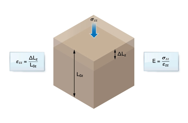
Young’s Modulus
Young’s modulus () is a measure of the resistance of a material to stress in the direction the applied stress. Young’s modulus is defined as:

Terms like stiffness or elastic modulus are often used as synonyms for Young’s modulus.
Figure 3 illustrates a geocell subjected to a uniaxial stress  illustrating the definition of Young’s modulus, .
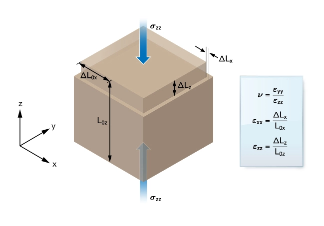
Poisson’s Ratio
Poisson’s ratio is named for the French mathematician, Simeon Poisson, who observed that when materials are compressed in one direction they tend to expand in a perpendicular direction. This is known as the Poisson effect. Poisson’s ratio () is defined as the ratio of the lateral expansion to the longitudinal shortening.

Poisson’s ratio describes the coupling between stress acting in one direction to deformation acting perpendicular to the applied load. For example, through the Poisson effect, gravitational stresses give rise to horizontal stresses.
Figure 4 illustrates a geocell subjected to a uniaxial stress σzz illustrating the definition of Poisson’s ratio, .
Bulk Modulus
The bulk modulus is a measure of a material’s resistance to volume change when subjected to a hydrostatic pressure  .
.
is defined as the ratio of the pressure to the volumetric strain.

Figure 5 illustrates a geocell subjected to hydrostatic pressure, , illustrating the definitions of bulk modulus and bulk compressibility  .
.
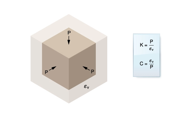
Compressibility
For isotropic materials, compressibility, , is the reciprocal of . Reservoir engineers tend to work in terms of compressibility (Figure 5).

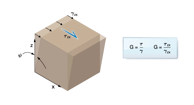
Shear Modulus
The shear modulus, , is a measure of a material’s resistance to shear strain,  , when subjected to a shear stress, (
 ).
).

Figure 6 is a schematic diagram showing the relationship of shear strain to shear stress.