Related Articles


Learning Objectives “Formation Anisotropy”
After completing this topic “Formation Anisotropy”, you will be able to:
- Describe common examples and causes of formation anisotropy for a range of different hydrocarbon reservoir types.
- Discuss the implications of electrical anisotropy for the interpretation of low resistivity pay zones.
By completing this course, and then applying the learnings in your job, you will be able to attain Basic Application Competence Level in the anisotropy aspects of low resistivity and low contrast pay interpretation.
Overview of Formation Anisotropy
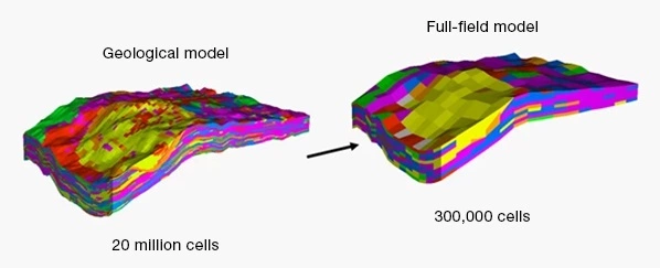
Many geological formations exhibit differences in some of their properties as a function of the direction in which the property is viewed. As examples, geophysicists have long recognized the directional differences in the velocities of compressional and shear elastic waves (Animation 1). Reservoir engineers also construct numerical simulation models of reservoirs (Figure 1) that exhibit differences in the directional permeability, normally as determined by special core analysis (SCAL) studies. Such changes with the direction are termed formation anisotropy.
Seismic reflection method
In the same way that many formations display directional variations in their seismic velocities or permeability, they often also exhibit changes in their resistivity with direction. Electrical anisotropy affects the overall resistivity in a low resistivity pay zone.
Defining Formation Anisotropy
A formation is considered to be anisotropic when the magnitude of a vector measurement of a given property changes with the direction. In many cases of formation anisotropy, the vector measurement effectively has a constant magnitude in all horizontal directions but exhibits a different magnitude when measured in the vertical direction.
Anisotropy is not the same attribute as heterogeneity. Anderson et al. (1994) offers two important distinctions:
- Anisotropy is defined as a variation in a vectorial value with direction at one point, whereas heterogeneity is defined by variation in vectorial or scalar values between two or more points within a given direction.
- Anisotropy tends to describe mainly physical properties, whereas heterogeneity is typically used to describe point-to-point variations in compositions, geometries or physical properties.
Scale
In “Oilfield Anisotropy: Its Origins and Electrical Characteristics,” Anderson et al. (1994) makes the following observation regarding the phenomenon of anisotropy.
“Fundamental to both anisotropy and heterogeneity is the concept of scale. Whether anisotropy and heterogeneity are perceived depends on sample size and sampling resolution. Anisotropy, for example, can be detected only when the observing wavelength is larger than the ordering of the elements creating the anisotropy (Helbig, K., 1994).”
While a crystal may be homogeneous above the molecular scale, it might be anisotropic when measured by the larger wavelengths of electromagnetic, or acoustic/sonic, propagation. An assemblage of crystals can form a homogeneous rock that is anisotropic if the crystals are aligned, or isotropic if they are randomly packed. When different layers of homogeneous and isotropic rock are measured as a single unit, they might be seen as heterogeneous and anisotropic (Anderson, et. al, 1994). Consider how scale might affect a laminated sandstone and shale formation, such as that shown in Animation 2, where the maximum thickness of each layer is 1 cm.
Finely laminated sandstone and shale sequence
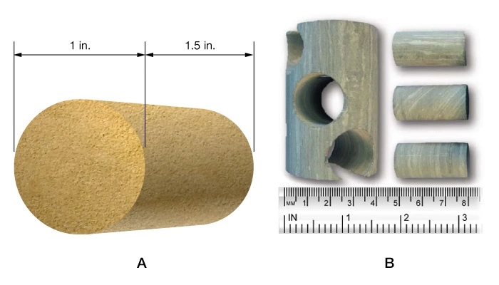
Because anisotropy depends on the perspectives of the sample size as well as the sample resolution, anisotropy on the scale of meters can sometimes escape detection in percussion (Figure 2A) and rotary (Figure 2B) sidewall core measurements. Anisotropy on the scale of centimeters might escape detection during the acquisition of vertically distributed pressure measurements by a wireline formation testing tool. In the former case, the wavelength is too small, whereas in the latter case, the data points may be relatively widespread.
Sedimentary Processes
Anisotropy often arises from processes that take place either during or after sediment deposition.
Anisotropy in Carbonates
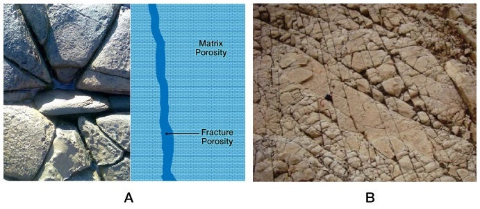
In many cases, anisotropy in carbonates is either controlled by fractures (Figure 3) or diagenesis, and, therefore, tends to take place after deposition. However, anisotropy in carbonates may also be attributed to changes in the carbonate mineralogy which are contemporaneous with deposition. These variations in mineralogy may be caused by changes in the carbonate content of the atmosphere and water, and can produce differences in the rock texture, porosity and permeability.
Anisotropy in Clastics
Anderson et al. (1994) state that the ultimate cause of deposition-related anisotropy in clastic formations is gravity. Movement of clastic grains begins under the influence of gravity.
At the bedding scale, anisotropy is attributed to two main factors:
- Periodic layering, which is usually attributed to changes in the sediment type, typically produces beds of varying material or grain size.
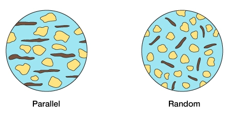
- Orientation of grains induced by the directionality of the transporting medium (Rajan, 1988). Upon settling, some grains tend to align in the direction of least resistance to the movement of the water and form parallel, as opposed to random, grain orientations. Platy, lenticular minerals, such as micas, are directionally aligned more easily than other minerals (Figure 4). In the left-hand image, the river current was moving from left to right
The azimuthal distribution of grain assemblages may also result from post-depositional tectonic deformation that causes shortening in one direction.
Shale Unconventional Reservoirs and Low Permeability Conventional Reservoirs
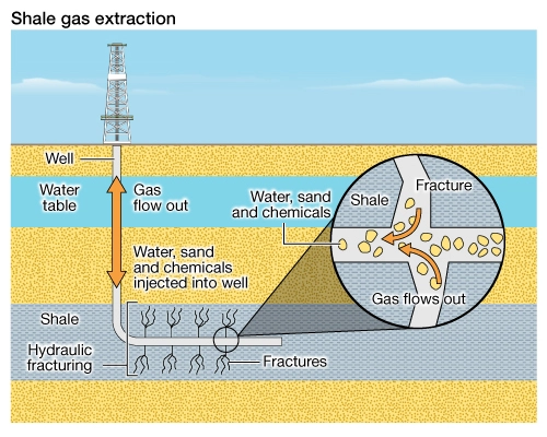
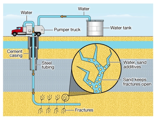
Grain alignments can create preferential rock stiffness in one direction, with relative weakness orthogonal to that direction (Lynn, 1991). This has a considerable significance for shale gas (Figure 5) and shale oil unconventional resources, as well as for some very low permeability conventional reservoirs, where the hydraulic fracturing of formations (Figure 6), often in conjunction with horizontal wellbores, is a pre-requisite for commercial hydrocarbon production. Often, development wells need to be directionally drilled, so that the optimum number of natural fractures can be encountered prior to their stimulation. It is vital to understand the formation anisotropy to enable the successful commercial development of these resources.
Diagenesis
There are several diagenetic processes that can result in formation anisotropy occurring after sediment deposition.
Diagenetic Processes Resulting in Formation Anisotropy
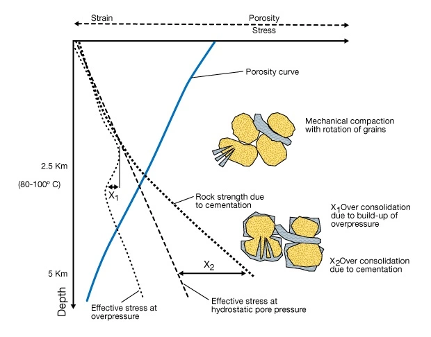
Compaction by overburden pressure results in the rotation of grain axes (Figure 7) (Manrique, 1994).
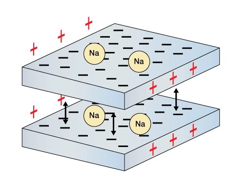
Alignment of clay platelets (Figure 8) caused by compaction and dewatering of the sediments results in anisotropy of shales.
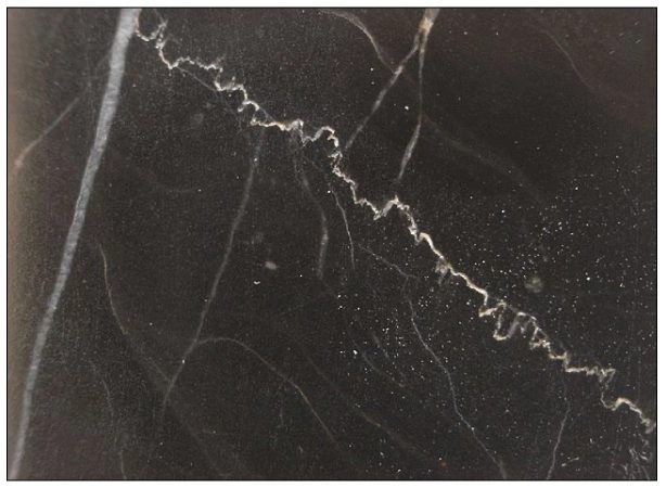
Pressure solution in carbonates can produce stylolites (Figure 9) of insoluble residue produced by dissolved material, which can act as laterally extensive flow barriers.
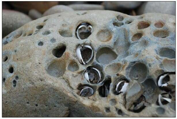
Burrowing (Figure 10) in carbonates or sandstones either increases or decreases depositional anisotropy.
Anderson et al. (1994) conclude that the process of diagenesis can significantly alter any anisotropies that were previously established during deposition.