Dry Air Drilling

14 minutes read

Typically layout of an air drilling site

Dry Air Drilling Overview

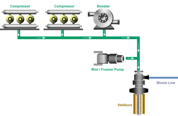
Dry air drilling is an old underbalanced drilling technique used primarily in environmentally sensitive areas to prevent formation contamination. A basic air drilling surface setup is shown in Figure 1.

Basic air drilling surface setup — **FIGURE 1**

However, effective hole cleaning is a problem with standard air drilling. The drag force on the cuttings has to be large enough to overcome the gravity required to move the particles up the hole. Most of the cuttings are obtained in the form of dust. The drag force on the cuttings increases with increasing air pressure and decreases with decreasing air velocity. Air temperature also influences density.

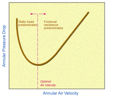
At high flow rates, cuttings move at more or less the same speed as the air. If the flow rate is decreased the frictional pressure drop decreases also, causing a drop in the efficiency of cuttings removal. The accumulation of cuttings eventually leads to a rapid pressure increase and reduced air circulation, which is known as “choking.” Choking velocity, as defined by Supon and Adewumi (1989), sets the limiting condition below which the cuttings are not supported by the air flow. Wellbore dimensions and projected circulation velocities must be carefully designed in order to keep velocities above the choking limit. Figure 2 shows the influence of air flow rate on annular pressure drop.

The influence of air flow rate on annular pressure drop — **FIGURE 2**

The air velocity decreases as the annular cross-section is increased. There is a high possibility that the cuttings will first start to accumulate around the top of the drill collars if the flow rate is not high enough to clean the well. The air velocity has to be at least equal to the cuttings settling velocity in order to transport the cuttings up the wellbore. The cuttings slip velocity can be estimated by Stokes’ law in consistent units:

Equation 1

$v_{sl} = \dfrac{1}{18}\left ( \dfrac{ds^{2}}{\mu} \right )\left ( \rho_{s}-\rho_{f} \right )g$

where:

v_sl = particle slip velocity

d_s = mean particle diameter

μ = fluid viscosity

ρ_s = particle density

ρ_f = fluid density

g = acceleration of gravity,

Which assumes that the cuttings are spherical. Stokes law is applicable only when Reynolds’ number is assumed to be below 0.1. The Reynolds’ number in field units is defined as:

Equation 2

$Re = 928\ \rho_{f}\ v_{sl}\ \dfrac{d_{s}}{\mu}$

where:

ρ_f = fluid density, lbm/gal

v_sl = particle slip velocity, ft/s

d_s = mean particle diameter, in

μ = viscosity, cp

If the air flow rate is in the turbulent region, which is most often the case, empirically defined friction factors must be used to obtain the particle slip velocity, as shown in the following equation:

Equation 3

$v_{sl}= 1.89\sqrt{\left ( \frac{d_{s}}{f} \right )\left ( \frac{\left ( \rho_{s}-\rho_{f}\right )}{\rho_{f}} \right )}$

where:

f = friction factor

The slip velocity increases with increasing particle diameter. This means that higher air flow rates are required to lift larger cuttings. The air density is controlled by local air pressure. Therefore, the air flow rate required to lift a certain size of cutting will increase with the square root of the bottomhole circulation pressure.

The increasing mass of air and cuttings in the annulus also causes an increase in frictional pressure drop. The Weymouth equation is a popular expression used to estimate the frictional pressure drop for gas flow in pipes. Angel modified the Weymouth equation using the concept of hydraulic radius of an annulus:

Equation 4

$f= \dfrac{0.14}{\left ( D_{h} - D_{p}\right )^{0.33}}$

where:

f = friction factor

D_h = wellbore diameter

D_p = drillpipe diameter

The last method was proposed for smooth pipe. While smooth pipe is not a valid assumption in most of the real cases, the method below should give more realistic results.

The friction factor can be determined using charts such as that presented by Bourgoyne et al. (1986). The following correlations presented by Fang et al. (2008) are more convenient to use:

$f = 10\wedge\left ( {A}'+{B}'\log \left ( N_{Re} \right )+{C}'\left [ \log \left ( N_{Re} \right ) \right ]^{2} \right )$

where

${A}' = 2.2954 - 2.2626 \Psi + 4.4395 \Psi^{2} -2.9825 \Psi ^{3}$

${B}' = -0.4193 - 1.9014 \Psi + 3.341 \Psi^{2} -2.0409\Psi^{3}$

$C' = 0.1117 + 0.0553\Psi - 0.1468\Psi^{2}+ 0.1145\Psi^{3}$

$N_{Re} = \left (\dfrac{124\ \rho_{f}\ v_{sl}\ d_{s}}{\mu } \right )$

where $N_{Re}$ is Reynolds number and $Ψ$ is particle sphericity, defined as the surface area of a sphere containing the same volume as the particle divided by the surface area of the particle.

The important practical information we need is the surface injection rate required for efficient cuttings removal, based on the relationship presented above. Several methods are available within the petroleum literature. However, none of them are easily applicable to full-scale field operations. Most of these techniques require some knowledge about the cutting size and shape, which is not easy to obtain.

The most widely used cutting transport analysis is based on the work of Angel, which was published in 1957. Angel suggested that efficient cutting transport at downhole conditions can occur if the kinetic energy of the air is equal to the air kinetic energy at standard conditions:

Equation 5

$\dfrac{1}{2}\rho_{min}\ v_{min}^{2} = \dfrac{1}{2}\rho_{std}\ v_{std}^{2}$

where:

ρ_min = gas density at minimum injection rate

v_min= gas velocity downhole

ρ_std = air density at standard conditions

v_std= minimum air velocity for efficient cuttings transport

The same expression can also be put into the following form:

Equation 6

$v_{min}= v_{std}\sqrt{\dfrac{\rho_{std}}{\rho_{min}}}$

By assuming that no slippage exists between cuttings and the air stream, Angel calculated the downhole pressure as a function of gas injection rate, hole diameter, drill pipe size and penetration rate. If slippage occurs, Angel’s equation underestimates the downhole pressure value, thus leading to monotonically decreasing air pressure values with decreasing flow rate. Another disadvantage of Angel’s formulation is that it uses the Weymouth equation to estimate the friction factor. Since borehole walls are very rough, the actual observed pressure drop is much higher than the estimate provided by Angel’s equation.

The results of Angel’s analysis are presented in a number of charts generated for different hole sizes, drill pipe diameters and penetration rates. These charts are widely used in estimating flow rate numbers in air drilling operations.

Annular Pressure

Comparison of Angel’s predictions with actual onsite measurements shows that some of the assumptions in Angel’s calculations are non-conservative, and lead to lower downhole air pressures. In order to overcome this drawback of Angel’s formulation, Guo et al. (1994) included Nikuradse’s friction factor equation in Angel’s formulation, resulting in a more accurate model.

Pressure Drop Around The Bit

An air drilling bit typically does not come with the nozzles used in mud drilling. The empty jet channel in the bit restricts the air flow, causing an increase in air velocity. When the air velocity reaches the speed of sound it cannot expand any further and the standpipe pressure becomes independent of the annular pressure. Under these conditions the air jet is known as “sonic”. In this case, pressure upstream of the bit is expressed as:

Equation 7

$P_{a}=0.00239\left [ \dfrac{Q\ T_{a}^{0.5}}{A_{n}} \right ]$

where:

P_a= pressure upstream of the bit, psia

Q= air flow rate, scfm

T_a= air temperature above the bit, ^oR

A_n= total area of bit nozzles, in²

For sub-sonic conditions the pressure is calculated by:

Equation 8

$P_{a}= P_{b}\left [ 1+\dfrac{0.236\ G^{2}\ T_{b}}{A_{n}^{2}\ P_{n}^{2}} \right ]^{3.5}$

where:

$G = \dfrac{Q\ \rho_{g}}{60}$

P_b = pressure beneath the bit, psia

T_b = air temperature beneath the bit, ^oR

Standpipe Pressure

Once the pressure above the bit is determined, any one of the existing friction factor relationships can be used to calculate the standpipe pressure. First, the flow regime has to be determined. Then for a relatively smooth pipe, the Weymouth equation can be used to represent the friction factor in order to get the standpipe pressure:

Equation 9

$P_{s}= \dfrac{P_{a}^{2} + \beta\ T_{av}^{2}\left ( e^{\frac{2\alpha h}{T}}-1 \right )}{e^{\frac{2\alpha h}{T}}}$

where:

$\alpha = \dfrac{S}{53.3}$

$\beta = \dfrac{\left ( 1.625\ \cdot \ 10^{-6}\ \cdot \ Q^{2} \right )}{D_{i}^{5.33}}$

D_i = internal diameter of the drill string, ft

S = gas gravity (1 for air)

T_av= average air temperature, ^oR

Depending the on the type of flow (sonic or sub-sonic), changes in annular pressure may or may not cause a change in standpipe pressure. Therefore, it is very important to follow standpipe pressure measurements closely.

Guo and Ghalambor (2002) have presented more accurate mathematical models for caclulating annular pressure, pressure drop across the bit, and standpipe pressure for vertical and deviated holes.

1 2 3 4 Next page

14 minutes read