Reservoir Fluid Flow and Natural Drive Mechanisms

54 minutes read

Water Drive and the Material Balance Equation

We refer to Havlena and Odeh (1963). The entire MBE equation is

$N_{p}\left [ B_{t}+\left (R_{p}-R_{si} \right )B_{g} \right ]+B_{w}W_{p}=N\, \left [ \left ( B_{t}-B_{ti} \right )+\dfrac{B_ti}{1-S_{wi}}\left ( S_{w}c_{w}+C_{r} \right )\Delta p+m\dfrac{B_{ti}}{B_{gt}}\left ( B_{g}-B_{gi} \right ) \right ]+W_{e}$

For saturated reservoirs, or when We is appreciable, or both, we can ignore compressibility of the rock and its associated water. The MBE becomes

$F=N\cdot E_{o}+Nm\dfrac{B_{ti}}{B_{gt}}\cdot E_{g}+W_{e}$ …………(49)

where:

F= total fluid withdrawals in reservoir volumes

E_o= total fluid withdrawals in reservoir volumes =B_t−B_ti, and

E_g= gas cap gas expansion =B_g−B_gi

Equation 49 has three possible unknowns: N, m, and W_e.

When the pressure is above the bubble-point, m = 0, and Equation 49 becomes

$F=N\cdot E_{o} + W_{e}$

$\dfrac{F}{E_{o}}=N+\dfrac{W_{e}}{E_{o}}$ …………(50)

Water influx is a function of time, pressure drop, and the physical properties of the aquifer, such as permeability, size, compressibility, porosity, and viscosity. We write

$W_{e}=C\, f\left ( t_{D},\ \Delta p \right )$ …………(51)

where:

C= constant

t_D= dimensionless time that includes actual time and the physical properties of the aquifer

$t_{D}=6.323\cdot 10^{-3}\left [ \dfrac{kt}{\phi \mu c_{e}A_{o}} \right ]$ where, ϕ, μ, c_e and A_o are aquifer properties)

Δp= pressure drop at the oil water interface.

Equation 50 indicates that if W_e (which is the parameter with the greatest uncertainty) is calculated correctly as a function of time, and a plot of $\tfrac{F}{E_{o}}$ versus $\tfrac{W_{e}}{E_{o}}$ is made on rectangular coordinate paper, a straight line should occur. The value of $\tfrac{F}{E_{o}}$ when $\tfrac{W_{e}}{E_{o}}$ =0 gives N, the initial oil in place. The calculations (Havlena and Odeh 1963, 1964) proceed as follows:

From the available data estimate the properties of the aquifer and calculate t_D as a function of a time interval, for example, at three, six, or nine months.
From production data calculate $\tfrac{F}{E_{o}}$ , and Δp at the selected time intervals.
Calculate f(t_D, Δp) of Equation 51 for the selected time intervals.
Plot $\tfrac{F}{E_{o}}$ versus $\left [\tfrac{ f\left (t_{D},\ \Delta p \right ) }{E_{o} }\right ]$ on rectangular coordinate paper.

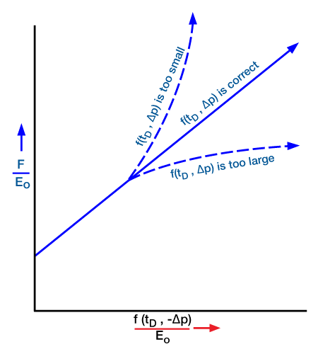
If the selected properties of the aquifer are correct (i.e., if Equation 51 is accurate) the plot will be a straight line (Figure 1).

Water Drive and the Material Balance Equation — **FIGURE 1**

The slope of the straight line is C, the water influx constant in Equation 51. The extrapolation of the straight line to

$\dfrac{ f\left (t_{D},\ \Delta p \right )}{E_{o}}=0$

gives the value of N. If the plotted points curve upward, the assumed water influx is too low; on the other hand, if they curve downward, the assumed water influx is too high. New values for the aquifer parameters must be assumed, and the calculations repeated until a straight line occurs. An example of this procedure is beyond the scope of this introductory module, but may be found in Havlena and Odeh (1963, 1964).