Porosity | What is porosity in well logging?

53 minutes read

porosity well log interpretation, porosity, well log, petrophysical evaluation, petrophysical interpretation

From Clean to Shaly Formations

Clean Formations

Density Porosity

For clean, water-bearing formations, and those formations where the shale volume is very close to zero, the density porosity can be generated from the bulk density log readings from either the logging while drilling (LWD) or wireline density logging tools, and the matrix and fluid densities using the equation:

$\phi _{(fractional)} =\dfrac{\rho _{ma} - \rho _{b}}{\rho _{ma} - \rho _{f}}$

or graphically by using Figure 1.

Porosity calculation from the bulk density for various formation matrix and pore fluid densities, Porosity calculation from the bulk density, porosity density, PHID, porosity, Borehole Wireline, Wireline Logging, well logging, What is porosity in well logging, What is a porosity log, Porosity definition, Well logging porosity, Types of porosity, Porosity measurement, Porosity calculation, Porosity logs, Effective porosity, Formation porosity, Porosity analysis, Porosity interpretation, Porosity determination, Porosity evaluation, Porosity in reservoirs, Petrophysical porosity, Porosity logging tools, Porosity estimation, Porosity models, Porosity control, Porosity saturation, Porosity data, Porosity variations, Porosity distribution, Porosity zones, Porosity anomalies, Porosity characteristics — **Figure 1**: Density porosity in clean, water-bearing formations using water base drilling mud

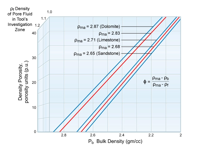
The matrix density in the most common conventional reservoir rocks varies between approximately 2.87 gm/cc for dolomite and 2.65 gm/cc for sandstone, with limestone at 2.71 gm/cc. The fluid density ranges from approximately 1 to 1.2 gm/cc for water base drilling muds, and from approximately 0.85 to 0.95 gm/cc for oil base drilling muds.

Neutron Porosity

Almost all neutron porosity logging tools are now run using a limestone matrix scale. Some neutron porosity logs have been historically, and a few still are, run on a sandstone scale. Figure 2 is a typical plot of the porosity measured by logging service companies’ compensated neutron porosity tools, using a limestone matrix against the true porosity for the indicated lines of constant lithology. All log acquisition service companies produce similar charts for their own particular tool designs, which are embedded in petrophysical evaluation programs for digital analyses.

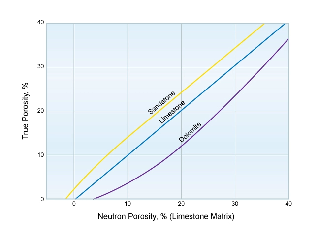
Such a chart, or its algorithm embedded in a log analysis computer program, can be used to convert to the true porosity if the actual lithology is known. When a pure limestone is logged with a neutron porosity tool run on a limestone matrix scale, no adjustment to the recorded neutron porosity is required to establish the true formation porosity, provided there are no light hydrocarbons or shale present.

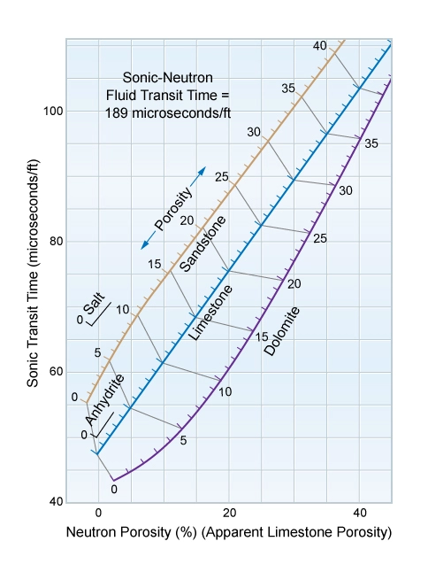
Sonic Porosity

Sonic porosity can be estimated with the Wyllie (1958) time average equation, using the interval transit time from the sonic log with the matrix and fluid travel times, as follows:

$\phi _s = \dfrac{\Delta t - \Delta t _{ma}}{\Delta t_f - \Delta t _{ma}}$

This is represented graphically in Figure 3.

Compaction factor correction chart, Travel paths of sonic pulses schematic, Sonic logging tool, sonic log, sonic porosity, porosity, well log, porosity log, Borehole Wireline, Wireline Logging, well logging, What is porosity in well logging, What is a porosity log, Porosity definition, Well logging porosity, Types of porosity, Porosity measurement, Porosity calculation, Porosity logs, Effective porosity, Formation porosity, Porosity analysis, Porosity interpretation, Porosity determination, Porosity evaluation, Porosity in reservoirs, Petrophysical porosity, Porosity logging tools, Porosity estimation, Porosity models, Porosity control, Porosity saturation, Porosity data, Porosity variations, Porosity distribution, Porosity zones, Porosity anomalies, Porosity characteristics — **Figure 3**: Wyllie time average equation for estimating sonic porosity

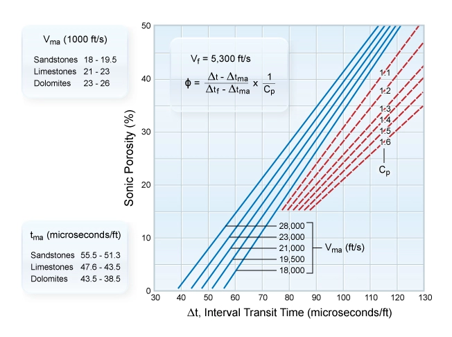
The interval transit time, Δt in microseconds/ft, is plotted against porosity. Lines on the chart correspond to various matrix velocities in ft/sec. Common conventional reservoir rocks have matrix velocities in the range of 18,000 ft/sec for sandstone to 26,000 ft/sec for dolomite, with limestone at around 22,000 ft/sec. Fluid velocities depend on the fluid type (oil, gas or water in the reservoir; flushed by, or mixed with, oil base or water base drilling mud filtrate, and the temperature, pressure and salinity of the fluids), but the range is usually from 4,300 to 5,400 ft/sec. The basic Wyllie equation is only accurate when the fluid in the pore space is water, or dead oil, the formation is compacted and the porosity is all intergranular. Dead oil is oil at such a low pressure that it contains no dissolved gas, or is a relatively thick oil or residue that has lost its volatile components.

In gas-bearing formations and formations with vuggy pore systems often found in dolomitic formations, the basic equation is often inaccurate for the determination of the total porosity and should not be used.

Unconsolidated formations do not conform to the basic Wyllie time average equation. A correction factor is required to compensate for the lack of formation consolidation. This correction factor is the term C_p, often known as the compaction factor, and the appropriate red dashed lines for compaction factors ranging from 1 to 1.6 are shown in Figure 3. The value of C_p is usually determined for a given formation from full diameter core analysis and existing sonic logs. An approximation technique uses the velocity of the nearest adjacent shales in microseconds per foot, divided by 100:

$C_p = \dfrac{\Delta t \ shale}{100}$

Some petrophysicists prefer to use the Raymer, Hunt and Gardner (1980) empirical transit time to porosity transform, usually termed the “Raymer-Hunt equation,” based on field observations.

$\phi _{\, log} = - \alpha - \left ( \alpha ^2 + \dfrac{\Delta t_{ma}}{\Delta t_{log}} - 1 \right )^{0.5}$

Where:

$\alpha = \dfrac{\Delta t_{ma}}{2\Delta t_{f}} - 1$

The Raymer-Hunt equation was introduced to correct for the observed anomalies and shortcomings of the Wyllie time average formula. The Raymer-Hunt equation gives generally slightly higher porosities than using the Wyllie formula. It provides improved porosity correlation over the entire porosity range and is applicable to consolidated formations. However, in high porosity, unconsolidated and uncemented rocks with slow velocities, neither the Wyllie nor the Raymer-Hunt empirical velocity to porosity transform may be adequate for a quality porosity determination.

Density-Neutron Crossplot

In cases where the lithology is very variable throughout the logged interval, or essentially unknown, no single porosity tool can effectively determine the formation porosity. Porosity can be better estimated by combining two porosity logs, especially the neutron porosity with the density logs.

Figure 4 shows a density-neutron crossplot, with the neutron porosity index plotted against the bulk density.

Density-neutron crossplot, porosity, porosity density, porosity, porosity combination, Borehole Wireline, Wireline Logging, well logging, What is porosity in well logging, What is a porosity log, Porosity definition, Well logging porosity, Types of porosity, Porosity measurement, Porosity calculation, Porosity logs, Effective porosity, Formation porosity, Porosity analysis, Porosity interpretation, Porosity determination, Porosity evaluation, Porosity in reservoirs, Petrophysical porosity, Porosity logging tools, Porosity estimation, Porosity models, Porosity control, Porosity saturation, Porosity data, Porosity variations, Porosity distribution, Porosity zones, Porosity anomalies, Porosity characteristics — **Figure 4**: Density-neutron crossplot

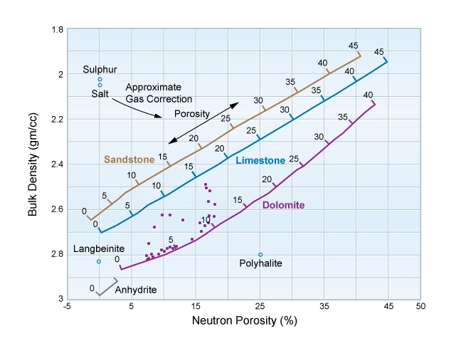
The lines of constant porosity are approximately straight lines, shown in gray in Figure 4, that are almost parallel to a NW-SE axis. Therefore, regardless of the actual formation lithology, readings of crossplotted pairs of ρ_b and ϕ_N establish the porosity of a clean formation within about one porosity unit. One limitation of the chart is that it assumes water-filled porosity. If the porosity is filled with hydrocarbons or oil base mud, additional corrections are required. The direction of a typical gas correction is shown, but its exact azimuth is largely a function of the gas density.

One method for making a quick approximation for the combination of neutron porosity and density porosity is to express ρ_b as an apparent limestone porosity, add this value to neutron limestone porosity, and divide by 2:

$\phi _{(N\textrm{-}D)} = \dfrac{\phi _{N\ (lime)} + \phi _{D\ (lime)}}{2}$

Where:

ϕ_N (lime) is the neutron porosity assuming a limestone matrix.

ϕ_D (lime)is the density porosity assuming a limestone matrix.

A slightly better approximation of the porosity can be made (regardless of the formation’s actual lithology) by combining the neutron limestone porosity with the density limestone porosity in the following manner:

Density-neutron combination porosity estimation = $\dfrac{\phi _N + 2\, \phi _D}{3}$

This porosity estimation technique works reasonably well even in gas bearing reservoirs, since it is a weighted average of density porosity and neutron porosity, which are affected by gas in opposite ways. In a gas bearing interval, the density porosity will be too high and the neutron porosity will be too low. Therefore, by taking a weighted average as shown, the gas effect is minimized.

However, both approximations result in overall poorer solutions to porosity determination than using crossplotting techniques.

Neutron-Sonic Crossplot

In rugose boreholes, the density log may be invalidated in those places where pad contact with the wellbore is lost. A sonic log may then be crossplotted with a neutron porosity log to estimate the formation porosity (Figure 5).

porosity, neutron porosity, sonic porosity, Borehole Wireline, Wireline Logging, well logging, What is porosity in well logging, What is a porosity log, Porosity definition, Well logging porosity, Types of porosity, Porosity measurement, Porosity calculation, Porosity logs, Effective porosity, Formation porosity, Porosity analysis, Porosity interpretation, Porosity determination, Porosity evaluation, Porosity in reservoirs, Petrophysical porosity, Porosity logging tools, Porosity estimation, Porosity models, Porosity control, Porosity saturation, Porosity data, Porosity variations, Porosity distribution, Porosity zones, Porosity anomalies, Porosity characteristics — **Figure 5**: Sonic-neutron crossplot

However, the constant porosity lines are not straight, as shown in gray in Figure 5. This results in a less reliable porosity estimation than can be obtained from a density-neutron crossplot, particularly with the presence of gas in the formation.

Shaly Formations

Single Porosity Tool Solutions

Shaly sandstones can be analyzed in several different ways. For example, a full diameter core sample may be analyzed to establish its porosity and grain density. Ideally, the application of the density porosity equation to such a sample reflects both laboratory measurements and bulk volume theory; i.e., if the sample is of bulk density ρ and the core analysis yields a grain density of ρ_gr, then:

$\rho = \rho _{gr}\, (1 - \phi _{core}) + \rho _{fluid} \cdot \phi _{core}$

thus:

$\phi _{core} = \dfrac{\rho _{gr} - \rho }{\rho _{gr} - \rho _{fluid}}$

If the same shaly sandstone sample had been logged by a density logging tool, the derivation of porosity would be more difficult, since the value of ρ_gr would be unknown. The matrix may be assumed to be a known rock type, such as quartz sandstone, and a default value used for its matrix density, ρ_ma. However, the shale content of the sandstone sample changes the effective grain density. This needs to be taken into account in establishing the bulk density versus porosity relationship.

The value of ρ_gr may be estimated if the fraction of clay solids and sand solids are known.

$\rho _{gr} = V_{clay} \cdot \rho _{clay} + (1 - V_{clay}) \cdot \rho _{sand}$

Where:

V_clay is the bulk volume of clay solids in unit volume of the shaly sandstone sample.

Thus, in clean sandstones, ρ_gr is numerically equal to ρ_sand, or ρma, at 2.65 gm/cc, and in shales ρgr is numerically equal to ρ_clay at close to 3 gm/cc. It should be recognized that shale densities are considerably less than 3 gm/cc, since a shale is composed of dry clay and water-filled pore space. For example, a 30% porous shale may have a bulk density of 2.4 gm/cc (0.3 ⋅ 1 gm/cc + 0.7 ⋅ 3 gm/cc). However, only a minute fraction of the pores are interconnected in the natural reservoir conditions. In this reservoir condition, the shale has close to zero permeability and requires hydraulic fracturing and horizontal production wells for commercial hydrocarbon production in unconventional reservoirs.

Log analysts have evolved many methods to handle the appropriate transforms from logging measurements to porosity in such cases. The following development is somewhat generalized.

If a generic porosity device P reads ϕ_P on the log and ϕPsh in the clay fillers and shale laminae, then the response of the device can be written:

$\phi _P = \phi + (1 - \phi - V_{sh}) \cdot \phi _{P \ matrix} + V_{sh} \cdot \phi _{Psh}$

Where:

V_sh is the bulk volume of the shale material

(1−ϕ−V_sh) is the bulk volume of the matrix

ϕ_P matrix is the tool’s response in pure matrix material

ϕ is the actual porosity

Assuming that ϕ_P matrix is zero, the relationship reduces to:

$\phi _P = \phi + V_{sh} \cdot \phi _{Psh}$

and, by rearrangement, to:

$\phi = \phi _P - V_{sh} \cdot \phi _{Psh}$

This generalized equation may be applied to each of the individual porosity devices. For the density tool, for example:

$\phi = \phi_{D(log)} - V_{sh} \cdot \phi _{Dsh}$

Typical values of ϕ_Dsh range from 25% to 0%, depending on the bulk density of the shaly materials. For example, if a density log reads 20% for the assumed matrix, and an independent shale volume indicator reveals that 30% of the bulk volume is occupied by shale (Vsh = 30%), which has an apparent density porosity of 15%, the equation can be written:

$\phi = 20 - 0.3\cdot 15 = 15.5\%$

In most cases, shaly formations appear more porous than they actually are.

For the neutron log, the equation may be written:

$\phi = \phi_{N(log)} - V_{sh} \cdot \phi _{Nsh}$

For the sonic log, it may be written:

$\phi = \phi_{S(log)} - V_{sh} \cdot \phi _{Ssh}$

The majority of values for ϕ_Nsh lie between 20% and 50%, and typical values for ϕ_Ssh are in a similar range.

Peeters and Holmes (2014) introduced a method for shaly sandstone petrophysical interpretation based on dry clay parameters. Dry clay volumes are derived from the difference of the apparent neutron porosity and density porosity in the total porosity system. Dry clay volume and dry clay parameters together determine the cation exchange capacities that are entered in the Waxman-Smits equation (Waxman and Smits, 1968). Clay types can be identified in cuttings or full diameter or sidewall cores.

Shale Unconventional Resource Reservoirs

Unconventional resource shale reservoirs are composed of a number of porosity types: effective porosity, clay porosity and micro-porosity associated with the shales, as well as hydrocarbon components such as the total organic carbon (TOC). The adsorbed hydrocarbons reside in the TOC component, and “free” hydrocarbons are in the effective porosity and the shale micro-porosity. Shale reservoirs have extremely low permeability, which requires hydraulic fracturing of the near wellbore region of horizontal wells to enable commercial hydrocarbon production rates and volumes (Orangi et al., 2011). Evolving horizontal well technologies, coupled with staged hydraulic fracturing, have made the development of a number of these reservoirs an economic reality.

For more detailed training about unconventional resource shale reservoirs, refer to the Shale course within this topic or the Introduction to Unconventional Resources topic.