Mathematical basin analysis models are mathematical representations of physical processes that occur in sedimentary basins. These models are used to simulate the behavior of sedimentary systems, including the transport, deposition, and erosion of sediment, and to predict the distribution and character of sedimentary rocks.
Introduction To Mathematical Basin Analysis Models
Tissot (1984) cites the development of “basin-scale geologic and geochemical modeling which allows a quantitative approach to the generation, migration, and entrapment of hydrocarbons” as having a major impact on exploration, enabling us to address subsidence history, heat flow, thermal and maturation history, and migration.
Welte and Yukler (1981) introduced an early quantitative model that combines geological, geophysical, geochemical, hydrodynamic, and thermodynamic data into a deterministic, dynamic basin model. They incorporate mass- and energy-transport equations, equations that describe the geochemical evolution of organic matter as a function of temperature, and empirical curves relating pressure and temperature, porosity and depth, and vitrinite reflectance to hydrocarbon generation. We use these equations and curves to compute pressure and temperature histories, the physical and thermal evolution of sediments, the maturation of organic matter, and hydrocarbon generation within a three-dimensional model of the basin. The results quantify hydrocarbon potential for source rocks at different stages of basin evolution.
Welte and Yukler begin their analysis using “all available data on sedimentary thicknesses, pressure, temperature, porosity, density, thermal conductivity, specific heat, maturity of organic matter, and amount of petroleum in place” to develop mathematical models that simulate the various petroleum-generating processes. Figure 1, (Steps in development of model of real-world system: [a] conceptual and mathematical models successfully represent the real system; [b] owing to poor understanding of real system, models are inaccurate.) shows the development of these models.
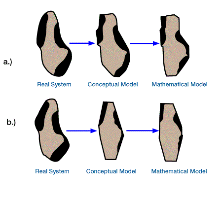
If data are sparse or poor quality, the models will not accurately represent the real system.
Available data are input into the model, which uses a set of non-linear partial differential equations of energy and mass balance to describe geological and geochemical evolution within a three-dimensional grid. The model simulates four basic units of the petroleum-generating system — geology, hydrodynamics, thermodynamics, and geochemistry (Figure 2, Input units for three-dimensional deterministic dynamic model).
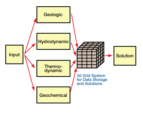
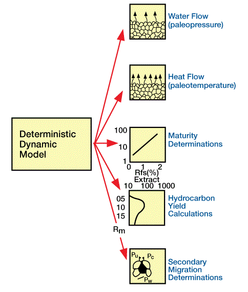
Table 1 and Figure 3 summarize output from these separate units.
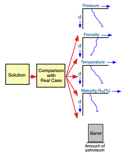
We then compare the output values to the actual measured values (Figure 4), and modify the conceptual model if the solution does not match reality.
| UNIT | OUTPUT |
|---|---|
| Geologic | Sediment type, source, depositional rates, etc. |
| Depositional environments | |
| Paleobathymetry | |
| Mineralogic evolution | |
| Tectonic Subsidence | |
| Hydrodynamic | Direction and rate of fluid flow |
| Hydraulic properties of fluids | |
| Porosity | |
| Pore pressure | |
| Potential migration pathways | |
| Thermodynamic Direction and rate of heat flow | |
| Thermal properties of fluids | |
| Thermal properties of sediments | |
| Geochemical | Type and amount of organic matter |
| Maturity of organic matter | |
| Generation potential of organic matter |
We can apply this modeling approach at any stage of basin exploration. In frontier areas, we will have to estimate many input data, but the model can be a good planning tool for new data collection. We update the input parameters as new data become available. In more mature areas, mathematical models can provide a new, quantitative perspective on hydrocarbon generation and distribution.
Figure 5,
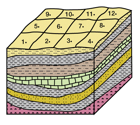
Figure 6,
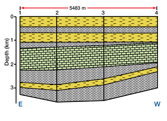
Figure 7,
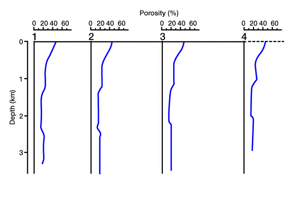
Figure 8, Figure 9
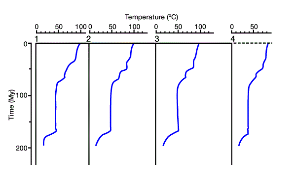
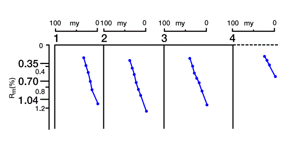
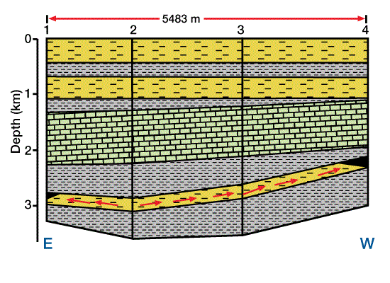
and Figure 10 show a simplified application to a generalized basin.
The block diagram in Figure 5 illustrates the basin geometry.
We generate a three-dimensional mathematical model to approximate the real setting. We then divide the three-dimensional model into a horizontally and vertically gridded cube. Geologic, hydrodynamic, thermodynamic, and geochemical data are defined at each grid point in the three-dimensional grid. Next, pore pressure, temperature, physical and thermal properties, maturation, and amount of hydrocarbon generation are calculated throughout the model. Secondary migration pathways are predicted and related to potential traps. Figure 6 shows a cross section through the mathematical model, with four locations marked for reference. Figure 7 shows the solution for porosity versus depth along the cross section at the four reference points, and Figure 8 shows time/temperature relationships at the same locations. The evolution of organic matter maturity is shown in Figure 9. Figure 10 shows potential secondary migration directions and potential trap locations.
This output gives us important information about the petroleum system. For example, the low porosity in the limestone units (Figure 7) forms a good top seal for the underlying units, creating a closed system of source and reservoir rocks. We can use time/temperature relationships (Figure 8) to predict source rock maturation at different times and locations within the basin (Figure 9), which we can then relate to the timing of trap formation.
This early basin summary shows how mathematical modeling can quantify the generation, migration, and accumulation of hydrocarbons. More advanced models have been developed and applied during the past decade. Ungerer et al. (1984) discuss five mathematical models that lead to “quantitative predictions of the geological phenomena leading to oil accumulations.” Each of the models (Figure 11 and Figure 12)
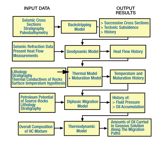
addresses a specific geological process:
- A backstripping model reconstructs of the sedimentary basin in time through successive cross sections.
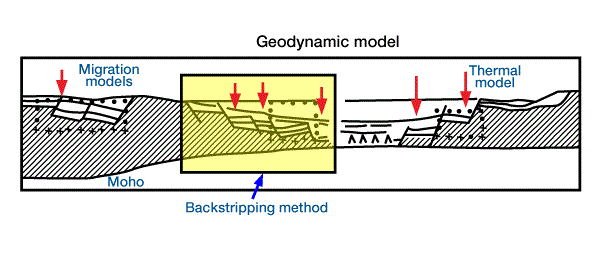
- A geodynamic model reconstructs heat flow histories used for basins formed by extension.
- A thermal model computes the temperature in the basin and is coupled to a kinetic model of organic matter maturation.
- A migration model computes the amounts of petroleum generated in the source rocks through time and the amounts accumulated in traps.
- A thermodynamic model determines the amount and composition of the hydrocarbons that may migrate in gaseous solution.
We can use the first three models to effectively analyze even poorly explored sedimentary basins. To apply the last two models, we need sufficient well control to provide adequate data on source rock distribution and richness.
 Petro Shine The Place for Oil and Gas Professionals.

