Logging Tools For Evaluating Low Resistivity And Low Contrast Pay

Specialized Logging Tools

Both logging while drilling (LWD) and wireline logging tools are continually evolving as technology progresses. In recent years, tools that address the problems caused by low resistivity pay zones have been developed. Technological specifications on these tools can be found at these leading oilfield technology companies: Baker Hughes, Halliburton, and Schlumberger.

Resistivity Tools

With advances in logging technology in recent years, the leading oilfield technology service companies have developed a number of new resistivity tools.

Resistivity Imaging Tools

Resistivity imaging tools were introduced as an evolution of dipmeter technology. Many of these tools have four or six (Figure 1) independent arms, each with articulating pads containing multiple electrodes. This combination of multiple pads and numerous electrodes results in vastly improved vertical resolution, down to fractions of an inch.

A typical tool emits an electrical current into the formation, while another current focuses and maintains a high-resolution measurement. The currents measured by each electrode vary according to the formation conductivity, which reflect changes in fluid properties, permeability, porosity, rock composition and grain texture. These variations are processed and converted into synthetic color images (Figure 2), which are interpreted according to the following convention:

• Light colors reflect low micro-conductivity zones of low porosity, low permeability, and high resistivity.
• Dark colors reflect high micro-conductivity zones of high porosity, high permeability, and low resistivity.

Resistivity Imaging Applications

Borehole resistivity imagers tend to use a fixed contrast presentation for gross correlations, and a dynamic averaging display to enhance the local geological and stratigraphic features:

• The static, or absolute, contrast allows the viewer to correlate color values between different zones of interest within the well, or between images from different wells.
• The dynamic averaging display is applied to local events to allow the viewer to distinguish features on a smaller scale, such as oil-filled porosity.

When integrated with other subsurface data, the images produced by a resistivity imaging tool enable the analyst to interpret laminated reservoirs and low permeability, shaly sandstones. The tool produces quantitative, high-resolution micro-resistivity measurements that aid in estimating the hydrocarbon saturation and the hydrocarbon in place in thin bedded reservoirs, thus improving the net pay estimation of laminated reservoirs.

Resistivity Imaging Services

Oilfield technology companies offer their own unique versions of resistivity imaging tools.

Halliburton Electrical Micro Imaging (EMI) Tool

The Halliburton Electrical Micro Imaging (EMI) tool has six independent arms, with an articulating pad on each arm (Figure 3). Each pad contains 25 sensors, with a resolution of 0.2 inch (5 mm). The central button on each pad produces high-definition, quantitative resistivity measurements with a depth of investigation comparable to a shallow-focused log. The tool is rated to 350ºF and 20,000 psi.

The EMI tool maps the formation’s micro-conductivity with its pad-mounted button electrodes. The current of each button is recorded as a curve, sampled at 0.1 inch (0.25 centimeters) or 120 samples per foot. The curves reflect the relative micro-conductivity variations within the formation. These current variations are converted to synthetic color or grey-scaled images. Light colors represent low micro-conductivity, while dark colors reflect high micro-conductivity zones.

Evaluating thinly bedded formations with a high-resolution resistivity curve will help to reduce the risk of miscalculating the hydrocarbon in place volumes. Figure 4 shows a comparison between a quantitative, high-resolution resistivity curve obtained from one EMI button (shown in track 3) and the digital focused log measurement (DFL) and the deep resistivity measurement (HDRS) curves (shown in track 4) acquired with the High-Resolution Induction tool. The neutron porosity and density log curves are displayed in track 5. Using the high-resolution resistivity measurement resulted in improved water saturation calculations and more realistic net pay estimations.

Schlumberger Formation MicroImager (FMI) Tool

In addition to a 24-button micro-electrical array pad on each of four arms, Schlumberger’s Formation MicroImager tool (FMI) (Figure 5) mounts an extendable pad below each arm to increase the pad coverage to about 80% of an 8-inch diameter borehole. The vertical resolution is 0.2 inch (5 mm) and the tool is rated to 350ºF and 20,000 psi.

Baker Hughes (STAR) Resistivity Imager Tool

The Baker Hughes STAR Resistivity Imager tool (Figure 6) acquires high-resolution images of borehole features that have resistivity contrasts. The six arms on the tool use a powered standoff to improve the pad contact with the borehole, thus providing resistivity coverage of 60% of an 8-inch diameter borehole. The tool is rated to 350ºF.

Schlumberger Azimuthal Resistivity Imager (ARI) Tool

Instead of relying on pad contact, the Schlumberger Azimuthal Resistivity Imaging (ARI) tool (Figure 7) uses an array of 12 azimuthal electrodes, spaced 30 degrees apart.

The dual laterolog array is able to measure the deep formation resistivity, but with a vertical resolution of only eight inches. As an imaging tool, the ARI is less sensitive to borehole rugosity than the FMI electrical imaging tool and can also provide coarse structural dip measurements. The tool was developed for the evaluation of heterogeneous reservoirs, thin bed analysis and fracture identification. It is rated to 350ºF and 20,000 psi.

Digital Array Induction Tools

Digital array induction logging tools use multiple receivers and multiple logging frequencies which provide capabilities that are not available with conventional induction tools. The main benefits of these tools are:

• Longer receiver coil spacings enable the determination of accurate deep resistivity, R_t, estimates, even in the presence of deep mud filtrate invasion.
• Short coil spacings provide information that is used to correct for borehole and near borehole effects.
• Better vertical resolution enables improved interpretations of thinly laminated, shaly sandstone sequences

Array Induction Applications and Services

The array induction device provides improved vertical resolution capabilities in thin beds. These measurements are used to evaluate complex reservoirs with beds of only 1 foot thickness or that have deep or unusual invasion profiles.

Baker Hughes High-Definition Induction Log (HDIL)

The Baker Hughes High-Definition Induction Logging (HDIL) tool generates an order of magnitude more data than some conventional induction tools. The HDIL tool investigates the formation at median depths of 10, 20, 30, 60, 90 and 120 inches, and is thus able to establish a precisely defined invasion profile. Identical readings by the 90-inch and 120-inch depth measurements are used to provide a direct indication of the true formation resistivity, R_t.

HDIL data can be processed in either of two modes, to optimally suit the reservoir conditions:

• HDIL true resolution data processing provides very accurate formation resistivity values by minimizing the effects that near-borehole features can have on deep reading resistivity curves. Using this format, the vertical resolution of the curves varies with the depth of investigation.
• HDIL resolution-matched processing is used in thin-bedded reservoirs, where bed boundary effects can limit the accuracy of deeper-investigating measurements. To improve interpretation in this situation, high-resolution data near the borehole are added to the deeper measurements so that all the curves are presented with the same matched vertical resolution of 1, 2 or 4 feet (Figure 8).

Schlumberger Array Induction Imager Tool (AIT)

The Schlumberger Array Induction Imager Tool (AIT) (Figure 9) uses eight induction coil arrays operating at multiple frequencies to generate five resistivity curves. The log curves have median depths of investigation of 10, 20, 30, 60 and 90 inches, and vertical resolution options of 1 foot, 2 feet and 4 feet.

Halliburton High-Resolution Induction Tool

The Halliburton/Baker Hughes High-Resolution Induction (HRI) tool features six radii of investigation at 90, 60, 50, 40, 30 and 24 inches. The log also displays a resistivity map to indicate the formation resistivity as a function of the depth and the radial distance from the HRI tool.

3D Multi-Component Resistivity Tool

Conventional induction logging tools use transmitter and receiver coils that are aligned with the long axis of the tool. In wells drilled perpendicular to the bedding, these tools measure the formation conductivity parallel to the bedding. When a reservoir is composed of thinly bedded, highly conductive shales and hydrocarbon-bearing sandstones that are below the vertical resolution of the tool, the measurements can produce a problematic low contrast, low resistivity pay effect. 3D multi-component tools overcome this interpretation challenge by generating both vertical and horizontal resistivity measurements.

Baker Hughes 3D Explorer Induction Logging Service (3DEX)

Baker Hughes developed a resistivity tool that is unique to the industry, which is designed to overcome the limitations of conventional induction tools in thin bedded, low resistivity, shaly sandstone formations. The Baker Hughes 3D Explorer Induction Logging Service (3DEX) provides both vertical and horizontal resistivity measurements independent of the borehole deviation and formation dip.

The 3DEX features three transmitter-receiver coil arrays, which are mounted orthogonally in the X, Y and Z planes relative to the tool axis. These coil arrays provide 3D coverage in their resistivity measurements:

• Two coils, XX and YY, measure resistivity in transverse directions, parallel to the tool body.
• A third coil, ZZ, measures resistivity in the direction of conventional resistivity tools, perpendicular to the tool body.
• In addition, there are cross-component measurements, XY and XZ.

These arrays induce currents that flow, for the most part, across laminated sandstone and shale sequences, and are far more sensitive to the hydrocarbon-bearing sandstone resistivity (Figure 10).

Inversion processing of the XX-YY-ZZ measurements obtained through the tool’s orthogonal coil configuration are used to determine the vertical resistivity, R_v, and horizontal resistivity, R_h. The 3DEX horizontal resistivity is always determined parallel to the bedding plane. The vertical resistivity is always measured perpendicular to the bedding plane. Therefore, regardless of changes in the borehole deviation or the formation’s apparent strike and dip, the 3DEX measurements of R_v and R_h remain properly oriented to the formation bedding. Where there is a difference in values between R_v and R_h, the formation is electrically anisotropic.

Electrical Anisotropy Effect

Conventional induction logging tools are limited to measurements in one dimension because their sensors are aligned along the length of the tool. Such measurements are only really satisfactory when formations are at least as thick as the tool’s vertical resolution.

In the presence of small apparent formation dips, the conventional induction tools induce currents that mainly flow in the highly conductive beds. Thus, when pay zones occur within thinly bedded sandstone and shale sequences, the conventional horizontal induction measurement is dominated by the lowest resistivity, which is usually found in the shale layers. As a result of this induced current flow pattern, the horizontal resistivity, R_h, is relatively insensitive to the higher resistivity of the hydrocarbon-bearing sandstones. In this manner, relatively small volumes of conductive shale can significantly reduce the apparent resistivity, thereby reducing the accuracy of the computed hydrocarbon saturations for the sandstone layers.

Vertical resistivity, R_v, is dominated by the highest resistivity component. In a hydrocarbon reservoir, R_v measurements provide more information on the resistive sandstone components, thus resulting in more accurate fluid saturations in the sandstone layers. The 3DEX tool capitalizes on this principle, with coil arrays aligned to resolve vertical resistivity.

In a thinly laminated sandstone and shale sequence, the effective horizontal and vertical resistivities are derived through parallel and series resistor models. The corresponding formulae are:

(Equation 1)

Where:

R_h= Horizontal resistivity

R_sh= Shale resistivity

R_sd= Sand resistivity

V_sh= Shale volume

V_sd= Sand volume

Such that

and

(Equation 2)

R_v= Horizontal resistivity

R_sh= Shale resistivity

R_sd= Sand resistivity

V_sh= Shale volume

V_sd= Sand volume

These equations are key to understanding the important differences between the horizontal and vertical resistivity.

Equation 1 helps to explain how the horizontal resistivity is affected by shale, or by sandstone:

• Horizontal resistivity, R_h, is strongly dependent on the low shale resistivity and the shale volume.
• Horizontal resistivity exhibits poor sensitivity to the sandstone resistivity.

Conventional induction tools, with their coils aligned along the length of the tool, are only able to measure perpendicular to the formation bedding, and thus are only sensitive to the horizontal resistivity.

Equation 2 demonstrates that the vertical resistivity averages the contributions from both the sandstone and shale, and thereby provides a much better indicator of thin, hydrocarbon-bearing sandstones.

The 3DEX tool capitalizes on the vertical and horizontal conductivity measurements to determine the laminar shale volume and the laminar sandstone conductivity. A Thomas-Stieber-Juhasz evaluation technique is applied to determine the volume of dispersed shale along with the total and effective porosities of the laminar sandstone fraction. By removing the laminar shale conductivity and porosity effects, the laminated shaly sandstone problem is reduced to a single, dispersed shaly sandstone model to which the Waxman-Smits equation can be applied.

Log Example

In this example from Mollison et al. (2001), the 3DEX tool was used to evaluate a shaly sandstone interval containing three distinct zones, each of which exhibit different ranges of electrical anisotropy and shale content (Figure 11).

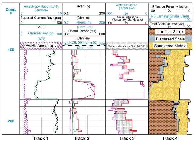
• The upper sandstone, from x100 to x145 feet, exhibits a fining upward sequence of moderately shaly sandstone. The data show significant electrical anisotropy in track 1, as demonstrated by the separation of R_v and R_h in track 2.
• The middle sandstone, from x145 to x169 feet, is a gas producing zone with low shale content. This interval exhibits little anisotropy, as would be expected in a massive, high porosity sandstone.
• The lower sandstone, from x169 to x220 feet, is characterized by higher shale content and higher electrical anisotropy than the upper sandstone. Conventional deep induction resistivity data, HDIL, shown in track 2, would not be able to effectively identify this interval as a potentially productive sandstone and shale sequence. However, the R_v and R_h data improve the evaluation accuracy of the lower sandstone and properly identify this as a finely laminated sandstone interval.

Petrophysical Evaluation of the Log

Directional resistivity measurements from the 3DEX tool can be used to compute both the volume of laminar shale and the resistivity of the sandstone fraction of a laminated formation without reference to other measurements or shale indicators. The 3DEX petrophysical evaluation model removes the laminar shale conductivity effects by utilizing the electrical anisotropy measurements, R_v and R_h.

In shaly sandstone sequences, the R_v and R_h measurements provide a close link to the petrophysical model through the direct computation of laminar shale. This laminar shale volume may be compared to Thomas-Stieber style volumetric laminar shale calculations, thus yielding a validation of the petrophysical models.

Petrophysical analysis of the example log reveals that the shales are predominantly laminar, with minor amounts of dispersed shale, as shown in track 4. In the upper sandstone interval from 100 feet to 145 feet, the calculated laminar sandstone resistivity, R_sd, is 3 to 5 ohm-m higher than that indicated by either the deep induction of the HDIL tool or the horizontal resistivity, R_h, of the 3DEX tool. The calculated water saturation, shown in track 3, from the laminar sandstone analysis is 10-15% lower than that obtained by standard water saturation analysis, indicating commercial hydrocarbon production rates are probable from this interval.

This comparison of laminar shale volumes may also provide valuable geological information. For example, the presence of anisotropic resistivity allows important additional interpretation as to the geometry of the layers. The lack of resistivity anisotropy could point to a lack of parallel bedding, such as is the case with disturbed, folded, or slumped bedding. Such intervals tend towards low deliverability.

The lower sandstone interval, from x169 to x220 feet, is the most interesting in this well, with the total shale volume in this interval being 60-70%. The separation between the R_v and R_h curves, together with the resulting anisotropy ratio, indicate that the formation is almost entirely laminar and thin bedded, with an average net to gross ratio of 35%. Water saturation through the laminar sandstone is calculated at 40-55%, which agrees well with the water saturation values calculated in the upper sandstone interval. The net result is a possible 18 feet of additional pay that might not have been identified by standard resistivity tools and traditional water saturation calculation methodology.

The 3DEX tool can also provide supplemental measurements for the High-Definition Induction Log (HDIL). It can be run simultaneously with the HDIL tool. Data processing at the wellsite is provided to expedite the decision-making process for potential drill stem testing and well completion.

Nuclear Magnetic Resonance (NMR) Tools

When microporosity, conductive mineralogy or altered framework grains are the cause of low resistivity pay problems, then nuclear magnetic resonance (NMR) is an alternative logging option. These tools do not depend on the rock conductivity and can be used to accurately determine the hydrocarbon saturation and distinguish between free water and bound water in the reservoir.

Conventional acoustic, density and neutron porosity logging tools are influenced by components of the reservoir rock. Because reservoir rocks typically have more rock framework than fluid-filled pore space, these conventional tools tend to be much more sensitive to the matrix materials than to the pore fluids.

Conventional resistivity logging tools, while being extremely sensitive to the fluid-filled space, are traditionally used to estimate the amount of water present in reservoir rocks and cannot be regarded as true fluid logging devices. These tools are strongly influenced by the presence of conductive minerals and, for the responses of these tools to be properly interpreted, a detailed knowledge of the properties of both the formation and the water in the pore space is required.

Nuclear magnetic resonance (NMR) logging tools use a permanent magnet to produce a magnetic field that excites the formation materials. An antenna transmits an oscillating magnetic field in precisely timed bursts of radio frequency energy into the formation. Between these pulses, the antenna is used to listen for the decaying echo signal from hydrogen protons that are in resonance with the field from the permanent magnet. Because this magnetic resonant frequency depends on the local strength of the magnetic field, the measurement zone of the tool is a function of the magnetic field generated and the radio frequency used.

NMR measurements respond primarily to hydrogen protons in the pore spaces of the formation, thus providing a measure of water or hydrocarbons in the rock. However, unlike neutron porosity measurements, the measure of NMR porosity does not include the hydrogen bound in the matrix of the rock, thus providing porosity values that are not influenced by the lithology. With only fluids visible to the NMR tool, it does not need to be calibrated to the formation lithology (Figure 12). This response characteristic makes NMR logging tools fundamentally different from conventional logging tools.

Unique Formation Measurements

NMR tools can provide three types of data, each of which makes these tools unique among well logging devices:

• Information about the quantities of fluids in the formation
• Information about the properties of these fluids
• Information about the sizes of the pores that contain these fluids

NMR tools are used to determine the total porosity, effective porosity, capillary bound water volume, free water volume, hydrocarbon volume and permeability. The basic physics behind NMR interpretation is common to all such data. Each of the current NMR logging service companies (Baker Hughes, Halliburton and Schlumberger) have their own proprietary interpretation methods. In addition, there are several companies that specialize in the interpretation of NMR data.

Schlumberger Combinable Magnetic Resonance Tool

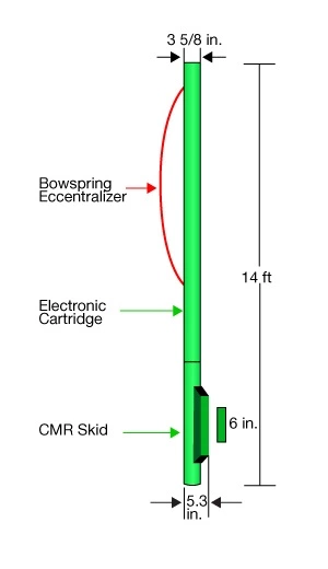
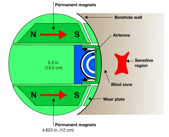
The Schlumberger Combinable Magnetic Resonance (CMR) tool (Figure 13) uses a directional antenna sandwiched between a pair of bar magnets to focus the CMR measurement on a 6-inch (15 cm) zone inside the formation. It is a compact, skid-mounted tool that is combinable with many other logging tools.

The vertical resolution of the CMR measurement makes it sensitive to frequent porosity variations, as is often seen in laminated shale and sandstone sequences. The sensitive region of the tool is shown in red in Figure 14. This region is approximately 0.5 × 0.5 by 6 inches long and is located about 1.1 inches inside the formation.

Baker Hughes Magnetic Resonance Imaging Log (MRIL) Tool

Baker Hughes’ Magnetic Resonance Imaging Log (MRIL) tool can be run in combination with other openhole logging instruments (Figure 15).

The tool needs to be run in a centralized configuration to ensure that the sensitive volume does not include the borehole fluid and is unaffected by the borehole rugosity. The MRIL measurements can investigate the formation at diameters of up to 18 inches. This tool can be operated simultaneously at different frequencies to increase the sensed volume, improve the signal-to-noise ratio, and allow multiple NMR measurements to be acquired simultaneously.

Halliburton Magnetic Resonance Imaging Log (MRIL) Tool

The Halliburton Magnetic Resonance Imaging Log (MRIL) tool can be tuned to be sensitive to a specific frequency, thereby allowing the MRI to image narrow slices of the formations (Figure 16).

The diameter and thickness of each thin cylindrical region are selected by specifying the central frequency and bandwidth to which the MRIL transmitter and receiver are tuned. The diameter of the cylinder is temperature dependent, but typically ranges from approximately 14-16 inches.

NMR Case Studies

Figure 17 shows a classic example of a low resistivity zone logged with conventional tools, which does not show any potential for future completion.

Figure 18 shows MRI and resistivity data provided by Halliburton, which was obtained in a low resistivity pay zone.

MRI Log Evaluation

On this log, there is a low resistivity sandstone interval from xx160 feet to xx260 feet. The interval is characterized by clean sandstone at the top, fining downward to shaly sandstone at the base. The average shale resistivity is 0.8 ohm-m. The maximum resistivity through the sand is 1.3 ohm-m at xx184 feet, and the minimum resistivity through that zone is 0.6 ohm-m at xx238 feet. The time domain analysis shown in track 5 indicates the presence of some free water, but the MRIAN model in track 6 shows the interval is water-free. In fact, this interval was tested at 2000 BOPD, with no water produced.