Sedimentary Basin Models

Sedimentary basin models are used in petroleum geology to understand the formation and evolution of sedimentary basins, which are the primary geological settings for the accumulation of oil and gas reserves. Sedimentary basins are formed through a combination of tectonic processes, such as rifting or subsidence, and the deposition of sedimentary layers over millions of years.

Quantitative Dynamic Stratigraphy

Stratigraphy now incorporates many topics normally assigned to other subdisciplines within the earth sciences, and we are in the midst of an evolution of stratigraphic analysis termed quantitative dynamic stratigraphy. In quantitative dynamic stratigraphy (QDS), we use quantitative techniques to analyze the geodynamic, stratigraphic and hydraulic attributes of sedimentary basins, treating them as features produced by the interactions of dynamic processes operating at specific times and places. Although QDS requires computer models that simulate processes in terms of natural laws and empirical generalizations, it is a much broader and more coherent approach to the analysis of sedimentary basins. QDS models are not inherently better than qualitative or conceptual models. Both are limited by the degree to which we understand process/response relationships, and by the degree to which we know the initial configurations and boundary conditions. However, describing a natural system in quantitative terms enables us to rigorously and systematically evaluate the concepts that led to the development of the model. QDS has numerous advantages:

• QDS enables us to more completely and effectively integrate knowledge from previously separate disciplines;
• it demands more accurate definition of the variables involved in and their operations upon the geologic system being simulated;
• it assesses or measures our confidence in the predictions made by
• it may lead to new insights by revealing previously obscure or unnoticed interdependencies and feedback mechanisms between processes and responses;
• it may force us to generate new explanations because model experiments may eliminate previously accepted explanations;
• through real-time simulations, it allows users to visualize and more completely understand interactions among processes and their responses; and,
• it reduces the time and effort that manual manipulation of data requires, enabling us to develop and test more hypotheses about geologic systems.

There is another overriding impetus for QDS — the need to increase the predictive capability, establish confidence levels, and assess the accuracy of sedimentary basin models in general. To successfully discover commercial accumulations of hydrocarbons, we must assess source, reservoir, seal, trap, maturation, migration and timing. Despite the recognized need to accurately assess these factors, most geological models are non-quantitative and limited in their predictability, and few provide a statement about confidence levels or the degree of accuracy of their predictions. Integrated QDS models provide the promise and technology to meet these needs.

Forward and Inverse Models

There are two general categories of quantitative models forward and inverse. Forward models make predictions, while inverse models solve for a model that best matches recorded observations (Figure 1).

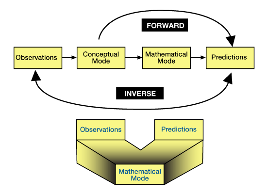
Forward models simulate sets of processes and responses — for example, open channel flow and sediment transport and deposition — that operate on a system having some specified initial condition and configuration — for example, topography, grain-size distribution and channel dimension. Given an initial configuration of a sedimentary basin, a forward model will simulate the evolution of that basin and predict its appearance and character at some later time. The accuracy of the model depends on: (1) the degree to which we understand the relationships and interdependencies between processes and responses; (2) our know-ledge of the initial and boundary conditions; (3) the similarity between the natural system and the set of algorithms, logic statements and mathematical expressions we use to represent that system; and, (4) the influence of randomness on the simulated processes.

In forward models, we progressively adjust the initial and boundary conditions and the process/response variables until the simulated results match available observations. If a forward model result matches the observations, we may then be able to use the model to simulate the geology between or beyond control points. However, different models can produce identical simulations, and this model may be only one of several possible models, each equally reasonable. There is no guarantee that a given model accurately represents the real world, even if the simulation results match the observed data.

In more formal terms, a model will satisy the condition of sufficiency if it produces a simulation that matches our recorded observations. But the model may not also satisfy the condition of necessity, since it may be only one of several potential models, each equally reasonable, that might produce identical simulations. We may judge different models producing different simulations to be non-unique in their accuracy and validity even after we compare their simulations with recorded observations, if those observations are uncertain, sparse, or of lesser resolution than model predictions.

Inverse models use present-day observations to estimate the initial and boundary conditions and the combinations of process/response variables that operated through time to produce the observed results. Inversion is a mathematically rigorous process of running a forward model multiple times, each time comparing model predictions with observations (Figure 2).

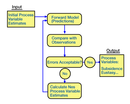
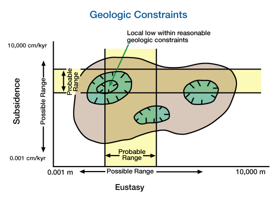
After each iteration, we adjust the forward model so that predictions based on the model more closely match the observations. In inversion, we can constrain the solution and estimate our confidence in the results by incorporating geologic data (Figure 3). These constraints can also help us develop accurate solutions when the response is non-unique.