Quick-Look Interpretation

17 minutes read

Overlays

Compatibly scaled overlays entail a comparison of two or more well logs. One curve is overlain on another via playbacks of the digital well log data and computer graphics displays so that the end result is a composite display with at least two curves. The relative deflection and separation between the two curves indicate a formation property of interest. An important aspect of overlays is that the curves being compared are compatibly scaled. Commonly used overlays include:

For hydrocarbon detection:

Spontaneous potential with R_xo/R_t
R_o versus R_t
Dielectric log-derived porosity with density porosity

For determining lithology, porosity and the presence of gas and fractures/vugs:

Neutron porosity with the density porosity
Density porosity with the sonic porosity

Spontaneous Potential With R_xo/R_t

This overlay is not universally applicable because it requires borehole conditions that result in the good development of the spontaneous potential (SP). In some cases, poor grounding prevents the acquisition of a usable SP log. In other cases, the similarity of the mud filtrate and formation water resistivities causes the SP log to have low amplitudes. However, where the appropriate conditions are met, it is an effective method for detecting hydrocarbons without needing to know the porosity.

The data inputs required are an SP, a deep resistivity log and a shallow resistivity log. The theory behind the method relies on Archie’s equation and the SP relationship:

$SP = -K\, \log \left( \dfrac{R _{mf}}{R_w} \right)$

Where:

R_w = the resistivity of the formation water.

R_mf = the resistivity of the mud filtrate.

K = a constant.

Archie’s equation, when written for both the invaded and uninvaded zones, allows the ratio of them to be calculated, eliminating F, the porosity-dependent formation factor:

$S_w^n = \dfrac{F \cdot R_w}{R_t}$

$S_{xo}^n = \dfrac{F \cdot R_{mf}}{R_{xo}}$

$\dfrac{S_w^n}{S_{xo}^n} = \dfrac{R_w}{R_{mf}}\cdot \dfrac{R_{xo}}{R_t}$

If an assumption is made that S_xo is related to S_w by the relationship:

$S_{xo} = \left( S_w \right)^{\frac{1}{5}}$

Then the quantity $\small \left( \frac{S_w}{S_{xo}} \right)^n$ can be replaced by $( \small S_w)^{\frac{5}{8}}$ , with the assumption that n is equal to 2.

Thus, the term $\frac{R_{mf}}{R_w}$ can be replaced by $\left( \frac{R_{xo}}{R_t} \right)\, (S_w)^{\frac{5}{8}}$ , and the SP equation rewritten as:

$-SP = K \, \log \left [ \left ( \dfrac{R_{xo}}{R_t} \right ) \left ( S_w \right )^{\frac{5}{8}}\right ]$

$-SP = K \, \log \left ( \dfrac{R_{xo}}{R_t} \right ) + K\, \log \left ( S_w \right )^{\frac{5}{8}}$

In a water-bearing zone where the water saturation, S_w, is 100%, the term $\small K\, \log \left ( S_w \right )^{\frac{5}{8}}$ is equal to 0. Consequently, the term $\small K \, \log \left ( \frac{R_{xo}}{R_t} \right )$ is numerically equal to -SP.

In an oil-bearing zone with the water saturation, S_w, being less than 100%, the term $\small K\, \log \left ( S_w \right )^{\frac{5}{8}}$ will be less than 1. Consequently, the term $\small K \, \log \left ( \frac{R_{xo}}{R_t} \right )$ will be numerically less than -SP.

Assuming that any SP reduction due to the presence of hydrocarbons is small, a comparison of the actual SP with $\small K \, \log \left ( \frac{R_{xo}}{R_t} \right )$ will have the following characteristics:

In clean, water-bearing zones, the two curves will track each other.
In hydrocarbon-bearing zones, the $\small K \, \log \left ( \frac{R_{xo}}{R_t} \right )$ curve will separate from the SP curve (Figure 1).

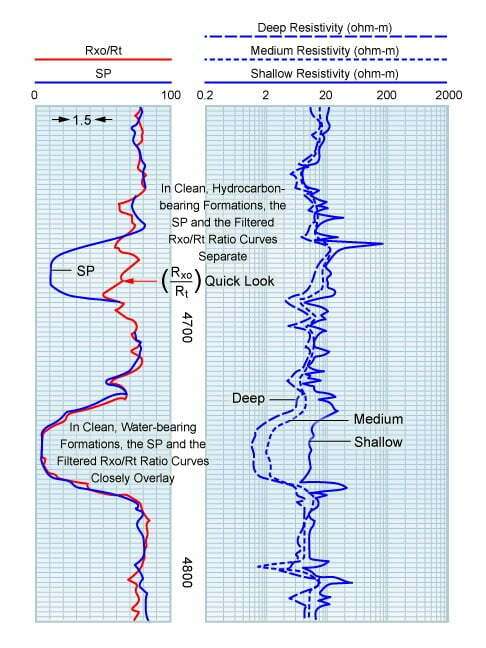
SP versus Rxo/Rt overlay playback, Quick-Look Interpretation — **Figure 1**: SP versus *Rxo/Rt* overlay playback

In the water-bearing lower sandstone formation of Figure 1, the SP and the filtered R_xo/R_t ratio closely overlay. In the hydrocarbon-bearing upper sandstone formation, the two curves separate. In shales, the R_xo/R_t ratio is close to 1, and so the R_xo/R_t and SP curves essentially overlay between depths of 4,685 and 4,710, and from 4,780 to 4,815.

In practice, some data manipulation is usually required to obtain a good overlay with the two traces overlaying in both the shales and the water-bearing zones. This requires using the correct K value for the formation temperature in question and the correct offsetting of either the SP baseline or the filtered R_xo/R_t curve.

In summary, this method works if there are sandstone and shale sequences with good SP development. This method cannot be used with oil base drilling muds, where the SP will be invalid.

Ro Versus Rt: The F Overlay

Another useful overlay for clean formations of known lithology is the F overlay, which effectively compares R_o with R_t.

The log analyst generates the formation factor, F, and then normalizes the logarithmic F curve with a logarithmic deep resistivity, R_t, curve so that these two curves overlay in clean, water-bearing zones. By so doing, the log F curve has been shifted by an amount equal to log R_w. Since the product of F and Rw is equal to R_o, the resultant effect is an overlay that compares R_o to Rt (Figure 2). Wherever the two curves separate, with R_t greater than R_o, the water saturation, Sw, is less than 100%, and, therefore, some hydrocarbons are present.

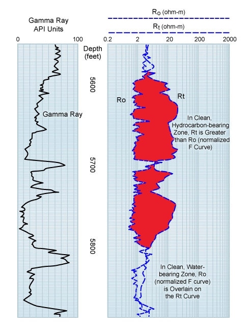
The F overlay, or Ro versus Rt, Quick-Look Interpretation — **Figure 2**: The F overlay, or *R_o* versus *R_t*

In the water-bearing section, the normalized F curve, being R_o, coincides with the R_t curve. In the hydrocarbon-bearing section, the R_t separates from Ro. This separation can be quantified in water saturation units by using an appropriate logarithmic scaler (Figure 3).

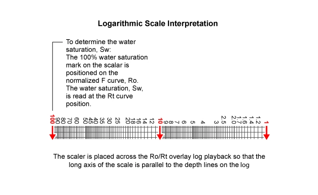
Logarithmic scaler concept, Quick-Look Interpretation — **Figure 3**: Logarithmic scaler concept

The scaler is placed across the overlay so that the long axis of the scale parallels the depth lines on the log. The 100% water saturation mark is placed on the normalized F curve, and the water saturation is read at the R_t curve position.

The formation water resistivity, R_w, does not need to be known beforehand. Normalizing the F curve to the deep resistivity in a water-bearing zone effectively computes the R_w.

The Logarithmic Movable Oil Plot

An extension of the F overlay technique is the logarithmic movable oil plot, which requires that two overlays be constructed: one to indicate the water saturation, S_w, of the uninvaded zone, and a second to indicate the water saturation of the flushed zone, S_xo. The result is a movable oil plot (MOP) on a logarithmic scale.

Generating the MOP is a two-stage process. First, the F curve is normalized to R_t in a water-bearing zone and the resulting R_o curve compared to the deep resistivity log. Secondly, the F curve is normalized to the R_xo in a water-bearing zone, and the resulting R_xoo curve, being R_xo in a rock 100% saturated with a fluid of resistivity, R_mf, is compared to the resistivity log (Figure 4).

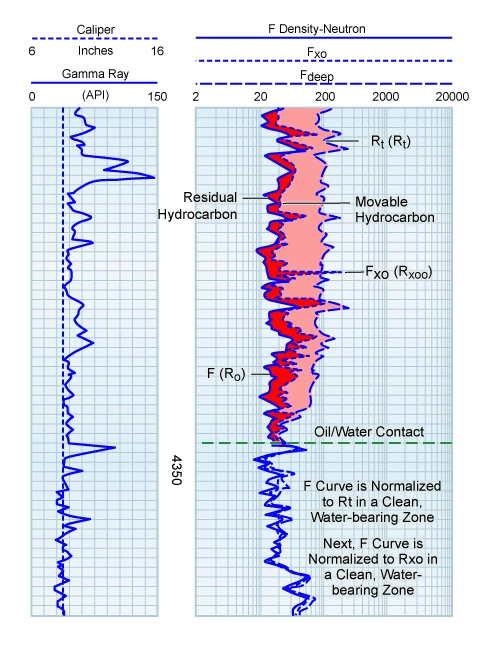
Logarithmic moveable oil plot MOP, Quick-Look Interpretation — **Figure 4**: Logarithmic moveable oil plot (MOP)

The area between the R_o and R_t curves is representative of the hydrocarbon-filled pore space. The MOP subdivides that volume into two parts, one denoting residual oil and the other movable oil.

Consider the bulk volume model shown in Figure 5.

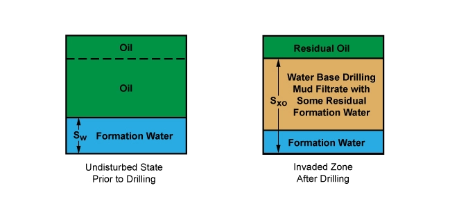
Bulk volume model, Quick-Look Interpretation — **Figure 5**: Bulk volume model

In the undisturbed zone prior to drilling, the saturating fluids are connate water and oil, and the water saturation is S_w. In the invaded zone after drilling, however, the saturating fluids are drilling mud filtrate, residual oil and a little residual connate water, and the water saturation is S_xo.

If Sxo is high as a result of the low residual oil saturation, then a large component of the oil in place has been flushed by the drilling mud invasion process. If S_xo is close to S_w, then very little of the oil in place has been moved, and the formation is potentially less productive. On the moveable oil plot, the area between the R_o curve and the Rxoo curve is a measure of the residual oil saturation. The area between the R_xoo curve and the Rt curve is a measure of the movable oil saturation.

The Neutron Porosity-Density Overlay

The neutron porosity-density overlay, usually the acquired log data or a playback, is a commonly used presentation, with the density and neutron porosity logs invariably run in combination both in logging while drilling (LWD) and wireline operational modes. Two types of overlay are considered here:

The compatible sandstone-scaled overlay for use in sandstone and shale sequences
The compatible limestone-scaled overlay for use in carbonate and evaporite sequences

The compatibly scaled sandstone presentation has the neutron porosity log on a sandstone matrix setting and is displayed on a 0% to 60% scale. Similarly, the bulk density recording must be converted to an apparent sandstone porosity curve by the choice of an appropriate value for the sandstone matrix density, such as 2.65 gm/cc, and displayed on the same scale as the neutron log (Figure 6).

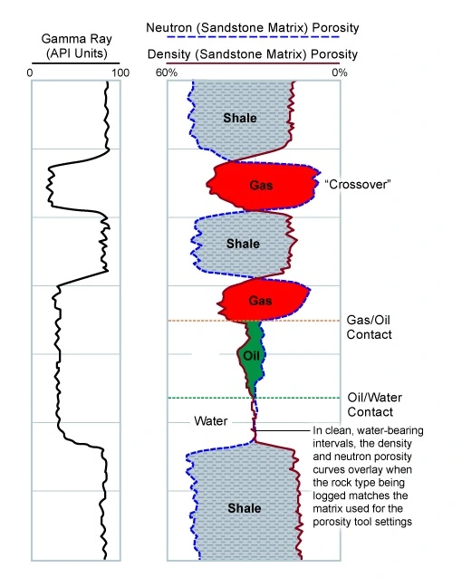
Density-neutron porosity overlay, Quick-Look Interpretation — **Figure 6**: Density-neutron porosity overlay/playback

In shales, the neutron porosity is much higher than the density log porosity. In clean, water-bearing intervals, the density and neutron porosity curves will overlay. In gas-bearing zones, the neutron porosity reads a lower apparent porosity than the density porosity. On this display, it is possible to quickly distinguish porous and permeable conventional resource reservoirs from shales, and to distinguish gas from water zones.

For carbonate reservoirs, the lithological mixture is limestone, dolomite and occasional evaporites. The compatible limestone presentation requires the neutron porosity log to be on a limestone matrix setting, with the density log on an apparent limestone porosity basis. Since dolomite and anhydrite may compute apparent porosities less than zero on a limestone matrix basis, an appropriate scale for this type of overlay is 45% to -15% (Figure 7), but occasionally a 60% to 0% scale is used. If the bulk density curve is used, rather than the computed density porosity, then the compatible scaling is 1.95 gm/cc to 2.95 gm/cc. In many parts of the world this limestone scaling is always used, irrespective of the actual formation lithologies.

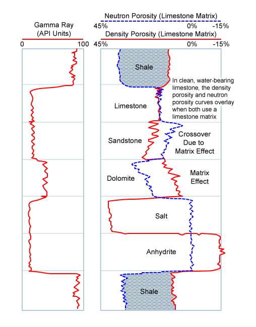
In clean limestone, the two curves overlay one another as the logs are acquired with limestone matrix settings. In dolomite, the apparent neutron porosity is higher than the apparent density porosity, and in sandstone the reverse is true. This sandstone crossover effect is due to the matrix effects on the two porosity devices and is a consequence of the limestone porosity scaling used. It should not be confused with crossover produced by the effect of gas, which significantly reduces the neutron porosity. In sandstone intervals, both curves have a similar character although separated from one another. If gas were present, it would be identifiable by an additional separation, with the neutron porosity even lower than the density.

The evaporitic salt and anhydrite intervals are also shown along with shale. Such a presentation is useful as a quick-look guide to the rock types drilled and is a very good starting point for other more detailed analysis.

Density-Sonic Overlay

The density-sonic overlay is useful for the detection of secondary porosity, which is often the result of vugs and/or fractures (Figure 8).

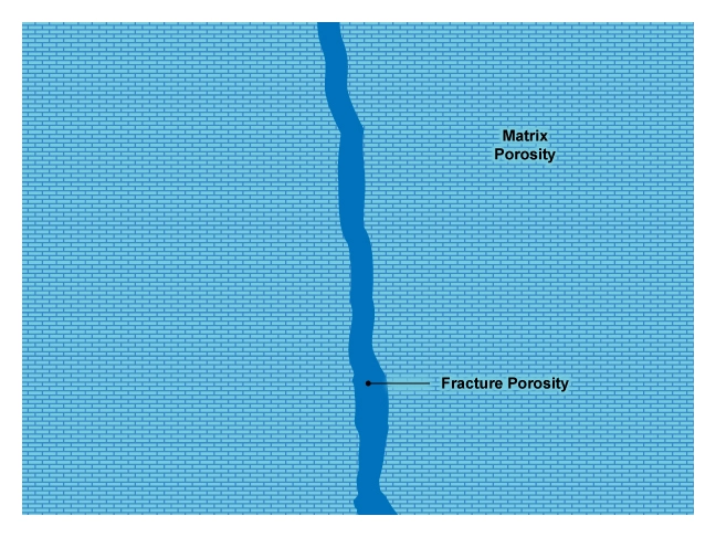
intergranular porosity and fracture porosity, Quick-Look Interpretation — **Figure 8**: Formation with both intergranular porosity within the matrix and fracture porosity

Provided the type of rock matrix is known, the density porosity will be equal to the total porosity:

$\phi _D = \phi _{total} = \phi _{matrix} + \phi _{secondary}$

The sonic logging tool, triggering as it does on the first compressional wave arrival, will only respond to the primary matrix porosity. Compressional waves traveling through a vertical, fluid-filled fracture, for example, will travel more slowly than those traveling through the adjacent rock matrix system. Because the sonic log response is triggered on the first arrival, the later arrivals passing through the fracture system will not be used to derive the sonic porosity. Thus:

[latex]\phi _{S} = \phi _{matrix}[latex]

In an overlay of the sonic porosity and the density porosity, ϕS and ϕD, the two curves separate in fractured or vuggy intervals (Figure 9), with the density porosity being higher by the amount of secondary porosity.

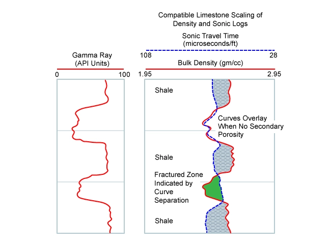
Density-sonic overlay indicating fracturing, Quick-Look Interpretation — **Figure 9**: Density-sonic overlay indicating fracturing

A number of scaling options are available. If the bulk density and the sonic travel time are to be overlain, then the compatible scaling is 1.95 to 2.95 gm/cc for the bulk density and 108 to 28 microseconds/ft for the sonic travel time.

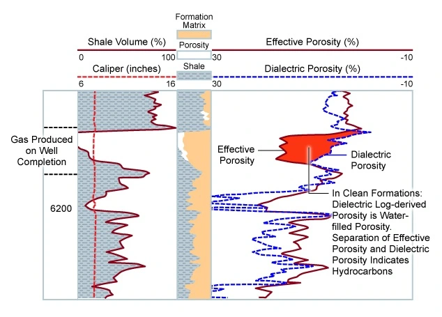
Dielectric Porosity Overlay

The compatible porosity overlay (Figure 10) of a dielectric log-derived porosity with another porosity curve is useful for quick-look hydrocarbon detection. The dielectric log-derived porosity is effectively the water-filled pore space, whereas a density porosity indicates the total porosity. If the formation is water-bearing, these two porosities will overlay. In hydrocarbon-bearing zones, separation will occur. The usual caveats of requiring clean formations and the correct choice of matrix parameters apply when computing these two porosities.