Log Analysis of Low Resistivity and Low Contrast Pays

34 minutes read

Log Calculations

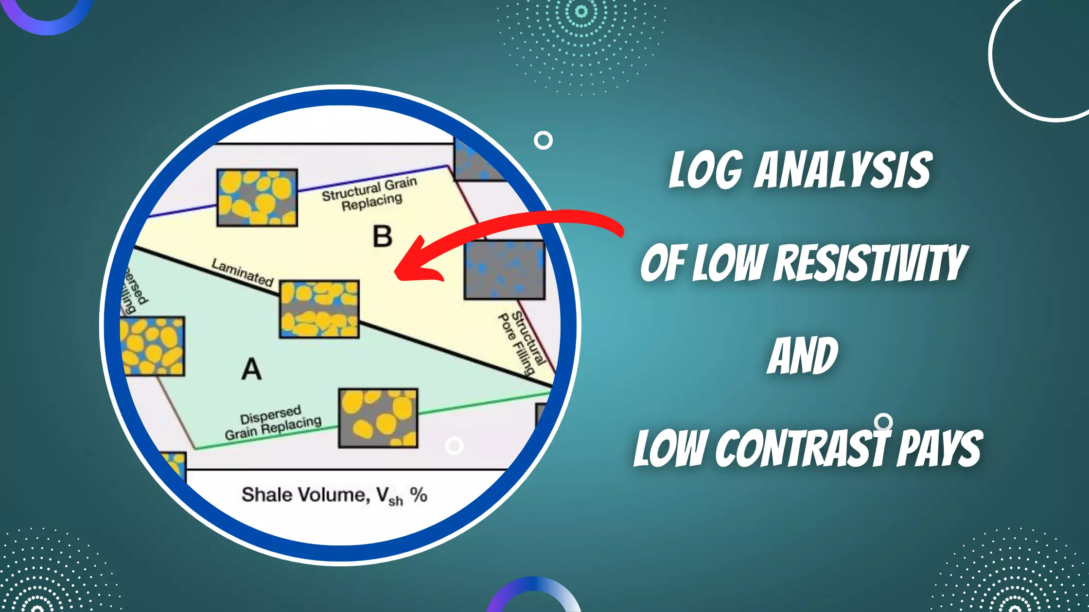
The primary cause of low resistivity pay is water and the clays and shales that attract and hold that water in place. Low resistivity is often caused by bound water, and such low resistivity should not automatically result in a well completed in that interval being a water producer. Various log evaluation methods have been devised to compensate for the presence of clay and shale to estimate a realistic value of the effective water saturation.

In most instances, the steps for correcting for the effects of clay and shale in both the porosity and water saturation calculations are:

Determine the volume of clay and shale, often termed Vshale (V_sh), in the formation.
Use the clay/shale volume to correct the total porosity values, and thus, calculate the effective porosity.
Use the clay/shale volume and the effective porosity to calculate the effective water saturation.

In general, clay and shale have the following effects on both LWD and wireline logging tools:

Sonic or acoustic porosity values read too high
Neutron porosity values read too high
Density porosity values read too high in many situations, except for deep burial and very high compaction of the clays
Resistivity values read too low

Step 1: Determining the Clay and Shale Volumes

Clay and shale volumes are normally derived from some combination of spontaneous potential (SP), natural gamma ray or spectral natural gamma ray, and crossplotted, or combined, neutron and density logs.

The various natural gamma ray logs, including spectral gamma ray logs, detect clay and shale by an increase in the natural gamma ray radiation.
The SP log detects clay and shale by a decrease in the SP deflection caused by the loss of ionic permeability in the shaly sections.
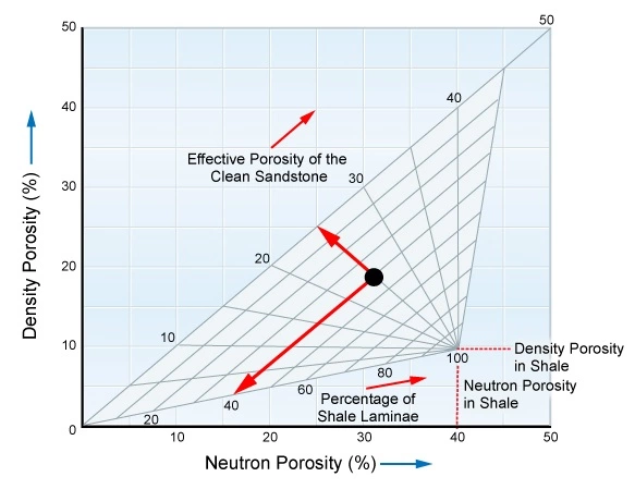
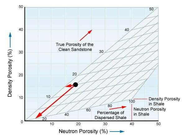
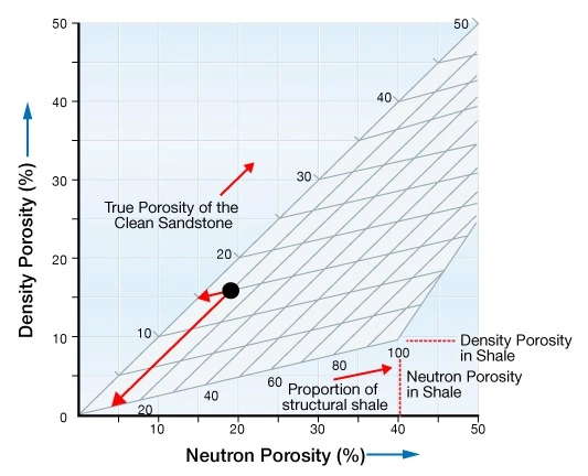
The neutron and density log, in combination, determine the shale volume by the use of the density-neutron crossplot. Figure 1, Figure 2, and Figure 3 show the crossplots for the three clay distribution models.

Shale volume determination in a laminated shaly sandstone, Log analysis of low resistivity and low contrast pays — **Figure 1**: Shale volume determination in a laminated shaly sandstone

Shale volume determination in a sandstone containing dispersed shale, Log analysis of low resistivity and low contrast pays — **Figure 2**: Shale volume determination in a sandstone containing dispersed shale

Shale volume determination in a structural shale model, Log analysis of low resistivity and low contrast pays — **Figure 3**: Shale volume determination in a structural shale model

Shale and Clay Volume from the Gamma Ray Logs

The most frequently used technique to derive the amount of clay and shale in a formation is by using the relative deflection of the gamma ray as a shale volume indicator. The simplest procedure is to rescale the gamma ray between its minimum and maximum values from 0% to 100% shale. The gamma ray index (I_GR) is used to linearly rescale the gamma ray between GR_min and GR_max.

Calculate I_GR:

$I _{GR} = \dfrac{GR _{log} - GR _{min}}{GR _{max} - GR _{min}}$

Where:

I_GR= Gamma ray index

GR_log= Gamma ray reading from shaly sand

GR_min= Gamma ray minimum from clean sand

GR_max= Gamma ray maximum from shale

Determine if the sand is consolidated or unconsolidated.
Use the I_GR value to calculate the clay and shale volume, dependent on whether the sand is consolidated or not:

$V _{cl} = 0.33 \cdot \left[ 2^{(2\cdot I _{GR})} - 1.0 \right]$ (for consolidated sands)

$V _{cl} = 0.83 \cdot \left[ 2^{(3.7\cdot I _{GR})} - 1.0 \right]$ (for unconsolidated sands)

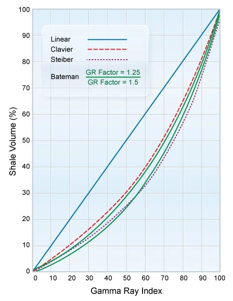
Alternatives for Estimating Shale Content from Gamma Ray Logs

Several studies indicate that the method of using the relative deflection of the gamma ray as a shale volume indicator does not always offer the best approach does not always offer the best approach as it tends to overestimate the formations shaliness, so alternative relationships have been proposed. The alternative relationships can be stated in terms of I_GR as follows:

V _{shale} = 1.7 - \left[ 3.38 - (I _{GR} + 7)^2 \right]^{\frac{1}{2}}

Relationship	Equation
Linear	$V _{shale} = I _{GR}$
Clavier	$V _{shale} = 1.7 - \left[ 3.38 - (I _{GR} + 7)^2 \right]^{\frac{1}{2}}$
Stieber	$V _{shale} = \dfrac{I _{GR}\cdot 0.5}{1.5 - I _{GR}}$
Bateman	$V _{shale} = I _{GR} \cdot (I _{GR} + GR \ factor)$

In the Bateman equation, the gamma ray factor is a number chosen to force the result to imitate the behavior of either the Clavier or the Stieber relationship. Figure 4 illustrates the differences in the calculated shale volumes between these alternative relationships.

Shale volume as a function of the gamma ray log reading, Log analysis of low resistivity and low contrast pays — **Figure 4**: Linear, Clavier, Bateman and Steiber gamma ray versus shale volume relationships

Not all clay and shale minerals are radioactive, and not all sandstones are non-radioactive. For example, because kaolinite contains no potassium, it would tend to mimic clean sandstone, if only the gamma ray log was to be used to determine the shale content. Conversely, when a gamma ray tool measures a sandstone containing a significant amount of potassium feldspars, the log will read higher and could potentially lead to the incorrect conclusion of more shale being present than was actually in the formation.

Clay and Shale Log Volume Calculations from SP Logs

Clay and shale volume can also be calculated from the spontaneous potential log:

$V _{cl} = 1.0 - \dfrac{PSP}{SSP}$

Where:

V_cl= Volume of clay

PSP= Pseudo-static spontaneous potential (SP reading in shaly sand)

SSP= Static spontaneous potential (SP in thick clean sand)

Clay and Shale Volume from Neutron and Density Log Combinations

The combination of neutron and density curves provides another method for estimating the clay and shale volume:

$V _{cl} = \dfrac{\phi _n - \phi _d}{\phi _{nsh} - \phi _{dsh}}$

Where:

V_cl= Volume of clay

ϕ_n= Neutron porosity in shaly sand

ϕ_d= Density porosity in shaly sand

ϕ_nsh= Neutron porosity of adjacent shale

ϕ_dsh= Density porosity of adjacent shale

If the shaly sandstone is gas bearing, then the shale volume should not be determined from the neutron density log, as the presence of gas will affect these logs, especially the neutron porosity.

Using the Lowest of the Clay and Shale Volume Estimates

The volume of clay and shale can be provisionally estimated by using all three methods described above, after which, the lowest estimate should be applied to shale corrections for porosity and saturation formulas because the various shale indicators will tend to overestimate the shale content.

Step 2: Using the Clay and Shale Volume Estimates to Correct the Porosity

The presence of clay and shale in a formation complicates the way in which porosity is calculated within the reservoir. Though the layer of closely bound surface water on the clay particle can represent a substantial amount of porosity, this porosity cannot be counted as part of a potential conventional resource reservoir for hydrocarbons. So, while a shaly formation may exhibit a high total porosity, it may only have a low effective porosity as a potential conventional hydrocarbon reservoir.

Techniques to Correct Porosity Logs for the Volume of Clay and Shale

Sonic Log

$\phi _e = \dfrac{\Delta t _{log} - \Delta t _{ma}}{\Delta t _{fl} - \Delta t _{ma}}\cdot \dfrac{100}{\Delta t _{sh}} - V _{cl} \cdot \left( \dfrac{\Delta t _{sh} - \Delta t _{ma}}{\Delta t _{fl} - \Delta t _{ma}} \right)$

Where:

ϕ_e= Effective porosity (acoustic log corrected for clay)

Δt_log= Interval transit time of shaly formation

Δt_ma= Interval transit time of the formation matrix

Δt_fl= Interval transit time of fluid (either 189 for fresh mud, or 185 for salt mud)

Δt_sh= Interval transit time of adjacent shale

V_cl= Volume of clay

Density Log

$\phi _e = \dfrac{\rho _{ma} - \rho _b}{\rho _{ma} - \rho _{fl}} - V _{cl} \cdot \left( \dfrac{\rho _{ma} - \rho _{sh}}{\rho _{ma} - \rho _{fl}} \right)$

Where:

V_cl= Volume clay

ϕ_e= Effective porosity (density log corrected for clay)

ρ_ma= Density of the formation’s clay-free matrix

ρ_b= Bulk density of shaly formation

ρ_fl= Density of fluid (1.0 for fresh mud and 1.1 for salt mud)

ρ_sh= Density of adjacent shale

Combination Neutron and Density Logs

$\phi _{nc} = \phi _n - V _{cl} \cdot \phi _{nsh}$

$\phi _{dc} = \phi _d - V _{cl} \cdot \phi _{dsh}$

$\phi _{e} = \dfrac{\phi _{nc} + \phi _{dc}}{2}$ for oil

$\phi _{e} = \left( \dfrac{\phi _{nc}^2 + \phi _{dc}^2}{2} \right)^{\frac{1}{2}}$ for gas

Where:

ϕ_e= Effective porosity (neutron and density logs corrected for clay)

ϕ_n= Neutron porosity of shaly formation

ϕ_d= Density porosity of shaly formation

V_cl= Volume of clay

ϕ_nc= Neutron porosity corrected for clay

ϕ_dc= Density porosity corrected for clay

ϕ_nsh= Neutron porosity of shale

ϕ_dsh= Density porosity of shale

Thomas-Stieber Method

Thomas and Stieber (1975) developed an interpretation model to quantitatively determine the shale content and distribution as an alternative to the linear, I_GR, method. This model relates variations in the gamma ray response to the concentration and distribution of shale. When this information is later combined with the porosity data, it is possible to determine the shale configuration, sandstone fraction and sandstone porosity.

This model works on the assumption that shaly sandstones and their interbedded shales are mineralogically similar to those shales above and below the sandstone. This will not be the case for the diagenetic alteration of feldspars into clay within the sandstones. The model was developed for geologically young sandstone and shale intervals but was not designed for complicated mineralogies involving carbonates.

Thomas and Stieber start by defining the relationship between the gamma ray count rates and the shale fraction. The shale models are divided into three distinct groups: dispersed, laminated, and structural.

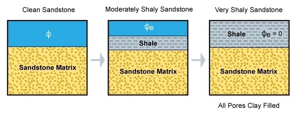
Dispersed Shale Model

For the dispersed shale model (Figure 5), Thomas and Stieber began by developing a formula to show that the observed gamma ray count rate is proportional to the amount of shale added to the pore system.

Dispersed clays progressively replacing porosity in a sandstone reservoir, Log analysis of low resistivity and low contrast pays — **Figure 5**: Dispersed clays progressively replacing porosity in a sandstone reservoir

According to their notation, the count rate, R, equals the count rate of sandstone, R_a, plus the count rate of shale, R_b, multiplied by the fraction of sandstone occupied by the shale, X_b:

$R = R_a + X_b \cdot R_b$

Where:

R= Count rate

R_a= Count rate of a solid block of sand material

X_b= Fraction of total rock volume occupied by dispersed shale

R_b= Count rate in shale

Applying this count rate to the gamma ray log, Thomas and Stieber relate to $\gamma$ , which correlates to porosity in terms of X_b, the bulk volume fraction occupied by shale. We can express the value of $\gamma$ in a sandstone stratum in terms of gamma ray readings:

$\gamma = \dfrac{GR _{shale} - GR _{log}}{GR _{shale} - GR _{sand}}$

$\gamma - 1 = \dfrac{V _{shale} - GR _{shale}}{GR _{shale} - GR _{sand}}$

The measure of sandstone radioactivity (ζ) is defined as:

$\zeta = \dfrac{GR _{shale}}{GR _{shale} - GR _{sand}}$

For dispersed shales, the relation between $\gamma$ and V_sh then becomes:

$V _{sh} = \dfrac{1 - \gamma}{\zeta}$

This can be expressed as:

$V _{sh} = \dfrac{1 - \phi _{shale}}{\left( \frac{GR _{shale}}{GR _{shale} - GR _{sand}} \right)}$

The minimum porosity available to the dispersed model occurs when shale completely fills all the original pore volume of the sandstone, or when X_b=ϕ_a.

The minimum dispersed porosity equals:

$\phi _a \cdot \phi _b$

Where:

ϕ_a= Porosity of sand

ϕ_b= Porosity of dispersed shale

When X_b>ϕ_a, then the relation between $\gamma$ an V_sh then becomes $\gamma = \small {1 - X_b} = \small {X_a}$

Laminated Shale Model

In the laminated shale model (Figure 6), shale is added to the sandstone stratum when a corresponding sandstone volume is filled with shale:

$\gamma = \dfrac{R_b - R_a - X_b \cdot (R_b - R_a)}{R_b - R_a} = 1 - X_b = X_a$

The count rate in the laminated model is actually the sandstone fraction.

Effect of changing the proportion of shale laminae on the amount of clean sandstone, Log analysis of low resistivity and low contrast pays — **Figure 6**: Effect of changing the proportion of shale laminae on the amount of clean sandstone

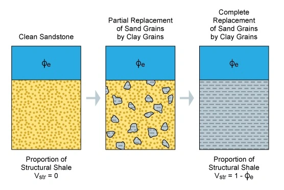
Structural Shale Model

In the structural shale model (Figure 7), the porosity increases with the amount of shale porosity that is added in place of the solid sand grains:

$R = (1 - \phi _a) \cdot Y\textrm{'} _a \cdot A_a - X_b \cdot (1 - \phi _a) \cdot Y\textrm{'} _a \cdot A_a + X_b \cdot (1 - \phi _b) \cdot Y\textrm{'} _b \cdot A_b$

Thomas and Stieber use the prime (‘) symbol to denote a change in counting yield due to a change in geometry in the material measured. In the structural model, the relationship between count rate and the shale volume is identical to that for the laminated model.

Structural shale model with the incremental replacement of sand grains by clay grains, Log analysis of low resistivity and low contrast pays — **Figure 7**: Structural shale model with the incremental replacement of sand grains by clay grains

Correlating Count Rates to Porosity

After Thomas and Stieber defined the relation between $\gamma$ and the shale fraction, they next constructed a theoretical $\gamma$ -porosity relationship based on the three models of shale distribution.

Dispersed Shale Model

Thomas and Stieber defined two relationships for dispersed shale:

Starting with pure sandstone, they added some amount of shale to that volume. Then Thomas and Stieber defined dispersed shale porosity as:

$\phi _{dis} = \phi _{sand} - V _{shale} \cdot (1 - \phi _{shale})$

In this case, where V_shale<ϕ_sand, the pore space is decreased by the amount of shale added (exclusive of the pore space contained in the shale).

When Vshale=0, then maximum ϕ_dis=ϕ_sand, and when V_shale=ϕ_sand, then minimum ϕ_dis=ϕ_sand⋅ϕ_shale. The relationship between count rate and porosity is:

$\phi _{dis} = \phi _{a} - \dfrac{1 - \gamma}{\zeta} \cdot (1 - \phi _b)$

Where:

ϕ_dis= Dispersed porosity

ϕ_a= Porosity of sand

ϕ_b= Porosity of shale

$\gamma$ = Count rate

ζ= Radioactivity of sand

For the second of the two relationships, Thomas and Stieber began with pure shale, added some amount of individual sand grains and then defined the dispersed shale porosity as:

$\phi _{dis} = \phi _{shale} - V_{sand} \cdot \phi _{shale} = \phi _{shale} - (1 - V_{shale}) \cdot \phi _{shale}$

In this case, total porosity is reduced by the amount of sand grains added:

$V_{shale} = \phi _{sand}$

The relationship between count rate and porosity is:

$\phi _{dis} = \phi _b - \gamma \cdot \phi _b$

when $\gamma = 0$ then $\phi _{dis} = \phi _{shale}$

Laminated Shale Model

For the laminated shale model, Thomas and Stieber replaced both the porosity and the solid rock fraction of the sandstone by shale porosity and the solid rock fraction of the shale:

$\phi _{lam} = \phi _{sand} - V_{shale} \cdot \phi _{sand} + V_{shale} \cdot \phi _{shale}$

The relationship between the count rate and porosity is:

$\phi _{lam} = \gamma \cdot \phi _a + (1 - \gamma) \cdot \phi _b$

When $\gamma = 1$ then $\phi _{lam} = \phi _{sand}$ and when $\gamma = 0$ then $\phi _{lam} = \phi _{shale}$

Structural Shale Model

In the structural shale model, the sandstone porosity is not changed but solid rock is replaced by an equivalent bulk volume of shale porosity:

$\phi _{str} = \phi _{sand} + V_{shale} \cdot \phi _{shale}$

The relationship between the count rate and porosity is:

$\phi _{str} = \phi _{sand} + (1 - \gamma) \cdot \phi _{shale}$

The maximum amount of structural shale which can be added equals the grain volume of the sandstone:

$V_{max} = 1 - \gamma _{min} = 1 - \phi _{sand}$

For structural shale models, the count rate is related to the porosity and radioactivity of the sandstone by the equation:

$\gamma = \zeta \cdot \phi _a$

Step 3: Calculating the Effective Water Saturation

Many water saturation equations have been proposed since Archie developed his original equation, some of which are detailed in Table 3.

Table 3: Some Commonly Used Water Saturation Equations
Poupon, et al. (1954)	$\frac{1}{R_t} = \frac{(1-V_{sh})\cdot S_w^2}{F\cdot R_w} + \frac{V_{sh}}{R_{sh}}$
Hossin (1960)	$\frac{1}{R_t} = \frac{V_{cl}^{2}}{R_{cl}} + \frac{1}{R_{tsd}}$
Simandoux (1963)	$\frac{1}{R_t} = \frac{S_{w}^{2}}{F\cdot R_w} + \frac{\varepsilon \cdot V_{sh}}{R_{sh}}$
Waxman and Smits (1968)	$\frac{1}{R_t} = \frac{R_w}{R_{tsd}}\cdot \left( \frac{1}{R_w} + \frac{B\cdot Q_v}{S_w} \right )$
Bardon and Pied – Modified Simandoux (1969)	$\frac{1}{R_t}=\frac{S_{w}^{2}}{F\cdot R_w}+\frac{V_{sh}\cdot S_w}{R_{sh}}$
Poupon and Leveaux (1971)	$\frac{1}{R_t}=\frac{S_{w}^{2}}{F\cdot R_w}+2\cdot \sqrt[]{\frac{V_{sh}^{2-V_{sh}}}{F\cdot R_w\cdot R_{sh}}}\cdot S_{w}^{2}+\frac{V_{sh}^{2-V_{sh}}\cdot S_{w}^{2}}{R_{sh}}$
Schlumberger (1972)	$\frac{1}{R_t}=\frac{S_{w}^{2}}{F\cdot \left ( 1-V_{sh} \right )\cdot R_w}+\frac{V_{sh}\cdot S_{w}}{R_{sh}}$
Clavier, et al. (1977)	$\frac{1}{R_t}=\frac{S_{w}^{2}}{F_o\cdot R_w}+\frac{\left ( C_{bw}-C_w \right )\cdot V_q\cdot Q_v\cdot S_w}{F_o}$
Juhasz (1981)	$\frac{1}{R_t}=\frac{S_{w}^{2}}{F\cdot R_w}+\left ( \frac{1}{F_{sh}\cdot R_{sh}}-\frac{1}{R_w} \right )\cdot \frac{V_{sh}\cdot \phi _{sh}\cdot S_w }{\phi }$

Table 3: Some Commonly Used Water Saturation Equations

Authors

Formula

Poupon, et al. (1954)

1Rt=(1−Vsh)⋅S2wF⋅Rw+VshRsh $\frac{1}{R_t} = \frac{(1-V_{sh})\cdot S_w^2}{F\cdot R_w} + \frac{V_{sh}}{R_{sh}}$

Hossin (1960)

1Rt=V2clRcl+1Rtsd $\frac{1}{R_t} = \frac{V_{cl}^{2}}{R_{cl}} + \frac{1}{R_{tsd}}$

Simandoux (1963)

1Rt=S2wF⋅Rw+ε⋅VshRsh $\frac{1}{R_t} = \frac{S_{w}^{2}}{F\cdot R_w} + \frac{\varepsilon \cdot V_{sh}}{R_{sh}}$

Waxman and Smits (1968)

1Rt=RwRtsd⋅(1Rw+B⋅QvSw) $\frac{1}{R_t} = \frac{R_w}{R_{tsd}}\cdot \left( \frac{1}{R_w} + \frac{B\cdot Q_v}{S_w} \right )$

Bardon and Pied – Modified Simandoux (1969)

1Rt=S2wF⋅Rw+Vsh⋅SwRsh $\frac{1}{R_t}=\frac{S_{w}^{2}}{F\cdot R_w}+\frac{V_{sh}\cdot S_w}{R_{sh}}$

Poupon and Leveaux (1971)

1Rt=S2wF⋅Rw+2⋅V2−VshshF⋅Rw⋅Rsh−−−−−−√⋅S2w+V2−Vshsh⋅S2wRsh $\frac{1}{R_t}=\frac{S_{w}^{2}}{F\cdot R_w}+2\cdot \sqrt[]{\frac{V_{sh}^{2-V_{sh}}}{F\cdot R_w\cdot R_{sh}}}\cdot S_{w}^{2}+\frac{V_{sh}^{2-V_{sh}}\cdot S_{w}^{2}}{R_{sh}}$

Schlumberger (1972)

1Rt=S2wF⋅(1−Vsh)⋅Rw+Vsh⋅SwRsh $\frac{1}{R_t}=\frac{S_{w}^{2}}{F\cdot \left ( 1-V_{sh} \right )\cdot R_w}+\frac{V_{sh}\cdot S_{w}}{R_{sh}}$

Clavier, et al. (1977)

1Rt=S2wFo⋅Rw+(Cbw−Cw)⋅Vq⋅Qv⋅SwFo $\frac{1}{R_t}=\frac{S_{w}^{2}}{F_o\cdot R_w}+\frac{\left ( C_{bw}-C_w \right )\cdot V_q\cdot Q_v\cdot S_w}{F_o}$

Juhasz (1981)

1Rt=S2wF⋅Rw+(1Fsh⋅Rsh−1Rw)⋅Vsh⋅ϕsh⋅Swϕ $\frac{1}{R_t}=\frac{S_{w}^{2}}{F\cdot R_w}+\left ( \frac{1}{F_{sh}\cdot R_{sh}}-\frac{1}{R_w} \right )\cdot \frac{V_{sh}\cdot \phi _{sh}\cdot S_w }{\phi }$

As Doveton (2001) observed, “the extension of Archie’s empirical model to shaly sandstones requires the evaluation of more elaborate, and frequently contentious, alternative models.”

The log interpretation methods described here are just a few of the numerous methods that now exist for determining water saturation of shaly sandstones (Figure 8).

Shaly sandstone sequence, Log analysis of low resistivity and low contrast pays — **Figure 8**: Shaly sandstone sequence

They are relatively simple to use and, with the exceptions of the Waxman-Smits and Juhasz equations, require only basic log data consisting of resistivity, SP, gamma ray, acoustic or sonic, neutron porosity and density LWD or wireline logs. These techniques account for the clay and shale in the formation.

When other contributors, such as heavy minerals, volcanics or other exotics, are thought to cause the low resistivity, then a more extensive suites of logs (including nuclear magnetic resonance, array induction and multi-component induction logs) can be used to investigate the problem. Furthermore, certain techniques have been developed for specific geographical areas of the world. In such cases, local knowledge should guide the selection of the appropriate log evaluation technique.

Dispersed Clay Method

Asquith (1990) states that the acoustic log detects the dispersed clay in the pore water as slurry and generates a porosity value that is equal to the sum of the volumetric fraction. The density log detects only water-filled porosity (Dewan, 1983). The fraction of the clean sandstone intergranular pore space occupied by clay is termed q:

$q = \dfrac{\phi _s - \phi _d}{\phi _s}$

Where:

ϕ_s= Acoustic porosity uncorrected for clay

ϕ_d= Density porosity uncorrected for clay

The effective water saturation equation is:

$S_{we} = \dfrac{\sqrt{\dfrac{0.8}{\phi _s^2}} \cdot \dfrac{R_w}{R_t} + \left( \dfrac{q}{2} \right)^2 - \dfrac{q}{2}}{1 -q}$

Where:

S_we= Effective (clay-corrected) water saturation

ϕ_s= Acoustic porosity uncorrected for clay

R_w= Formation water resistivity

R_t= Deep formation resistivity

$q = \dfrac{\phi _s - \phi _d}{\phi _s}$

An important aspect of the dispersed clay model is that the equation does not require a value for the shale resistivity, R_sh, or the volume of clay, V_cl, because the shaly factor, q, is determined within the shaly sandstone.

The effective porosity equation is:

$\phi _e = \left( \dfrac{\rho _{ma} - \rho _{b}}{\rho _{ma} - \rho _{fl}} \right) - V_{cl} \cdot \left( \dfrac{\rho _{ma} - \rho _{sh}}{\rho _{ma} - \rho _{fl}} \right)$

Where:

ϕ_e= Effective porosity corrected for clay

ρ_ma= Matrix density

ρ_b= Bulk density from shaly sand

ρ_fl= Fluid density

ρ_sh= Shale density

V_cl= Volume of clay

The dispersed clay method for determining water saturation may be unreliable in gas-bearing sandstones because the density porosity may be greater than the acoustic porosity.

Fertl Method

This method, developed by Walter Fertl, can be used for dispersed clays or when the clay or shale distribution is unknown, because this equation does not require a value for the shale resistivity, and thus, avoids the risk of plugging in an R_sh value from an adjacent shale bed that might not represent the actual shale resistivity within the shaly sandstone. (Asquith notes that the difference in resistivities between dispersed clay in the reservoir and the resistivity of the adjacent shale is especially pronounced when resistivity of the adjacent shale is greater than the resistivity of the shaly sandstones.)

$S_{we} = \dfrac{1}{\phi _d} \cdot \left[ \sqrt{\dfrac{R_w}{R_t} + \left( \dfrac{\alpha \cdot V_{cl}}{2} \right)^2} - \dfrac{\alpha \cdot V_{cl}}{2} \right]$

Where:

S_we= Effective (clay-corrected) water saturation

ϕ_d= Density porosity uncorrected for clay

R_w= Formation water resistivity

R_t= Deep formation resistivity

V_cl= Volume of clay

α= 0.25 in the Gulf Coast or 0.35 in the Rocky Mountains

The effective porosity is derived from neutron and density logs that have been corrected for clay and shale content.

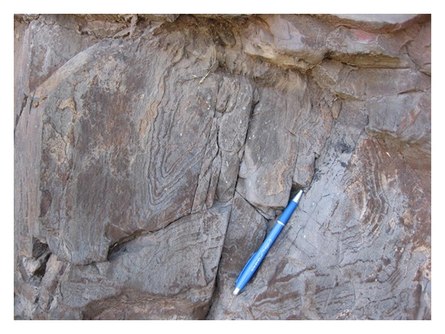
Simandoux Method

Water saturation equations that require a shale resistivity component, R_sh, will generate higher water saturations than those provided by the standard Archie equation when the resistivity of the adjacent shale is greater than the resistivity of the shaly sandstone.

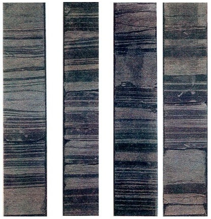
In general, the $\frac{V_{sh}}{R_{sh}}$ term is appropriate only in laminated shaly sandstones. Therefore, whenever it has been established that the shale distribution is laminated (such as by reviewing slabbed full diameter cores [Figure 9]), it is advisable to use either the Simandoux method or the dual water method, which is discussed later in this subject.

Finely laminated shaly sandstone formation outcrop, Log analysis of low resistivity and low contrast pays — **Figure 9**: Laminated shaly sandstone sequence displayed as a slabbed full diameter core

The reason for restricting the value of R_sh to laminated shaly sandstones is that clays in the shaly laminated sandstone and the adjacent shale are both depositional in origin and, thus, may differ significantly in resistivity:

$S_{we} = \dfrac{C\cdot R_w}{\phi _e^2} \cdot \left[ \sqrt{\dfrac{5\cdot \phi _e^2}{R_w\cdot R_t} + \left( \dfrac{V_{cl}}{R_{sh}} \right)^2} - \dfrac{V_{cl}}{R_{sh}} \right]$

Where:

S_we= Effective (clay-corrected) water saturation

ϕ_e= Effective porosity corrected for clay

R_sh= Resistivity of adjacent shale

R_w= Formation water resistivity

R_t= Deep formation resistivity

V_cl= Volume clay

C= 0.40 sandstones and 0.45 for carbonates

The neutron and density porosities are corrected for clay and shale to obtain the effective porosity, ϕ_e, using the method described by Dewan (1983).

Modified Simandoux Method

The Simandoux equation was later fine-tuned as more case studies with dispersed shale were completed and real data was incorporated:

$S_w = \sqrt{\left( \dfrac{F \cdot R_w}{R_t} \right) + V_{sh} \cdot \left( \dfrac{F \cdot R_w}{2\, R_{sh}} \right)} - V_{sh} \cdot \left( \dfrac{F \cdot R_w}{2\, R_{sh}} \right)$

Where:

S_w= Water saturation

F= Formation factor

R_w= Formation water resistivity

R_t= True resistivity

R_sh= Resistivity of adjacent shale

V_sh= Volume of shale

Dual Water Model

The dual water model (Clavier et al., 1977) works on the basis of partitioning the pore water into bound water and free water, each of which contributes to the resistivity of the shaly sandstone. The bound water and the free water have their own associated resistivities, R_b and R_w respectively. In this model, R_b is fresher than R_w, which can move freely within the pores. Following is a summary of the dual water formulation:

1. Calculate the volume of clay and shale, as previously described.

2. Correct the neutron and density porosities for the effects of clay and shale.

$\phi_{dc}= \phi _d - V_{cl} \cdot \phi _{dsh}$

$phi _{nc}= \phi _n - V_{cl} \cdot \phi _{nsh}$

Where:

V_cl= Volume of clay

ϕ_d= Density porosity

ϕ_n= Neutron porosity

ϕ_nc= Neutron porosity corrected for clay

ϕ_dc= Density porosity corrected for clay

ϕ_dsh= Density porosity of shale

ϕ_nsh= Neutron porosity of shale

3. Calculate the effective porosity

$\phi _e = \dfrac{\phi _{nc} + \phi _{dc}}{2}$ oil zone

$\phi _e = \left( \dfrac{\phi _{nc}^2 + \phi _{dc}^2}{2} \right)^{\frac{1}{2}}$ gas zone

Where:

ϕ_e= Effective porosity corrrected for clay

ϕ_nc= Neutron porosity corrected for clay

ϕ_dc= Density porosity corrected for clay

4. Calculate the total porosity of the adjacent shale.

$\phi _{tsh} = \phi _{dsh} + \phi _{nsh}$

Where:

ϕ_dsh= Density porosity of shale

ϕ_nsh= Neutron porosity of shale

5. Calculate the total porosity and the bound water saturation.

$\phi _{t} = \phi _e + V_{cl} \cdot \phi _{tsh}$

$S_b = \dfrac{V_{cl} \cdot \phi _{tsh}}{\phi _t}$

Where:

S_b= Clay-bound water saturation

ϕ_t= Total porosity

ϕ_e= Effective porosity

V_cl= Volume of clay

ϕ_tsh= Total porosity of adjacent sahle

6. Calculate the bound water resistivity from the adjacent shale.

$R_b = R_{sh} \cdot \phi _{tsh}^2$

Where:

R_b= Bound water resistivity

R_sh= Resistivity of adjacent shale

Asquith warns that the shale resistivity, R_sh, is only equal to the resistivity of the clay in the shaly sandstone when the clay in the sandstone is allogenic. When the effective water saturations calculated from equations that require R_sh are much higher than the effective water saturations calculated from equations that do not require a value for R_sh, then dispersed authigenic clay is probably present.

7. Calculate the apparent water resistivity, R_wa, in the shaly sand.

$R_{wa} = R_t \cdot \phi _t^2$

Where:

R_wa= Apparent water resistivity

R_t= Deep formation resistivity

ϕ_t= Total porosity

8. Calculate the total water saturation corrected for clay

$S_{wt} = b + \sqrt{b^2 + \dfrac{R_w}{R_{wa}}}$

Where:

S_wt= Total water saturation corrected for clay

$b = \dfrac{S_b \cdot \left( 1 - \dfrac{R_w}{R_b} \right)}{2}$

R_w= Formation water resistivity

R_wa= Apparent formation water resistivity

9. Calculate the effective water saturation, S_we, of the shaly sandstone

$S _{we} = \dfrac{S_{wt} - S_b}{1 - S_b}$

Where:

S_we= Effective water saturation

S_wt= Total water saturation

S_b= Clay bound water saturation

Waxman-Smits Method

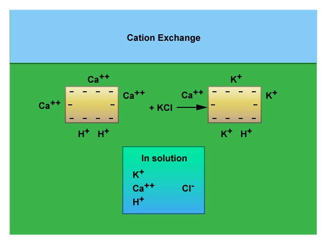
Crystal surfaces absorb water using their ion exchange sites (Figure 10). Different minerals have different cation exchange capacity (CEC) values.

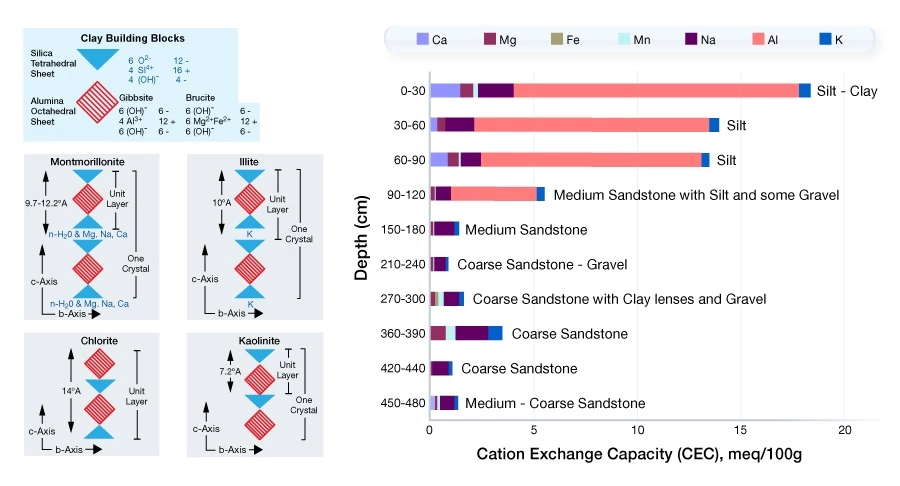
Cation exchange illustration, Log analysis of low resistivity and low contrast pays — **Figure 10**: Cation exchange illustration

Quartz, as the major constituent of sandstone, has practically no CEC, but illite and montmorillonite (Figure 11), because of their high specific surface areas, have high CEC values. Thus, CEC is a mechanism by which clay can suppress the formation’s resistivity, causing lower values of the petrophysical parameters m and n, but if the cation exchange capacity is ignored, there is the risk of estimating water saturations that are erroneously high. This may cause hydrocarbon productive zones to be overlooked or result in low hydrocarbon-in-place estimates.

Building blocks of clays (left), and cation exchange schematic for some common clays (right), Log analysis of low resistivity and low contrast pays — **Figure 11**: Building blocks of clays (left), and cation exchange schematic for some common clays (right)

A water saturation equation was developed by Waxman and Smits (1968) to express the water saturation, S_w, in shaly sandstones as a function of the cation exchange capacity of the clay disseminated in the sandstone:

$S_w = \sqrt[n^*]{\dfrac{F^{^*} \cdot R_w}{R_t \cdot \left( 1 + \dfrac{R_w \cdot B \cdot Q_v}{S_w} \right)}}$

Where:

$F^{^*} = F_a \cdot (1 + R_w \cdot B \cdot Q_v)$

$Q_v = \dfrac{CEC \cdot (1 - \phi)\cdot \rho _{ma}}{100 \cdot \phi}$

S_w= Formation water saturation

R_w= Formation water resistivity

R_t= True formation resistivity

F^∗= Formation resistivity factor independent of clay conductivity $= \frac{a^*}{\phi ^{m^*}}$

F= Formation resistivity factor

n^∗= Saturation exponent independent of clay conductivity (slope of RI versus S_w plot)

B= Specific counterion activity, $\mathrm{\frac{\left( \frac{1}{ohm-m} \right)}{\left( \frac{equiv}{liter} \right)}}$

Q_v= Quantily of cation exchangeable clay present, $\mathrm{\frac{meq}{ml}}$ of pore space

CEC= Cation exchange capacity, $\mathrm{\frac{meq}{100\, gm}}$

ρ_ma= Grain density or raock matrix, $\mathrm{\frac{g}{cm^3}}$

a= Tortuosity coefficient (intercept on F versus ϕ plot)

m^∗= Cementation exponent (slope of F^∗ vs ϕ plot)

ϕ= Measured porosity, fraction

The Waxman-Smits equation requires an iterative solution because S_w appears on both sides of the equation. This method, although based on sound laboratory measurements and good petrophysical principles, lacks one vital factor for its regular application the ability to derive CEC values from conventional well log measurements. Correlations for a given oil or gas field can be made between core measurements of CEC and other log measurements. However, the cores must be measured first. There is no practical means of using this method if only well log data are available.

Because shale conductivity is a function of the cation exchange capacities of the various types of clay minerals and their abundances, shale conductivity is influenced more by the surface area of the clay minerals than by the volume of the clay minerals. Experimental data confirms that fine grained clays exhibit higher exchange capacities than coarser grained forms of the same volume. Doveton notes that all shale indicators estimate the volume of the shale component but are not able to provide an explicit assessment of the grain size or clay mineralogical variation. Thus, without a tool that measures the CEC directly, it is difficult to design log analysis procedures that accommodate the cation exchange capacity data. Asquith (1990) notes that another objection to the Waxman-Smits equation is that it predicts that the effective water resistivities will decrease as water sandstones of constant formation water resistivity, R_w, become shalier, a point which Clavier et al. (1977) dispute with evidence to the contrary.

The dual water model devised by Clavier et al. (1977) circumvents some of the flaws found in the Waxman-Smits model and is indirectly based on the CEC.

Juhasz Method

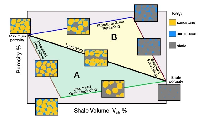
Juhasz (1981) developed a system for assessing the shale distribution and determining the average shaliness, porosity and hydrocarbon saturation of shaly sandstone laminae. This system is derived partially from the relationship between the total porosity and shale volume described by Thomas and Stieber (1975), as well as the Waxman-Smits (1968) saturation model. Juhasz uses crossplots of the porosity versus shale volume to evaluate the formation (Figure 12).

Two triangles make up the porosity versus shale volume crossplot, Log analysis of low resistivity and low contrast pays — **Figure 12**: Two triangles make up the ϕ versus *V_sh* crossplot

The overall evaluation process has been split into separate procedures to cover the total porosity system, as well as the effective porosity system.

Shale Distribution within the Total Porosity System

Juhasz uses the pattern and position of data points within the total porosity versus volume shale crossplot to evaluate the formation (Figure 13).

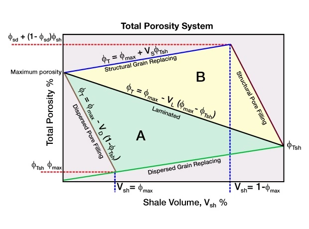
Total porosity versus shale volume crossplot, Log analysis of low resistivity and low contrast pays — **Figure 13**: Total porosity versus shale volume crossplot

The positions of the lines used in the crossplot are based on the maximum clean sandstone porosity and the total shale porosity observed in the zone being evaluated. Juhasz assumes that only the combination of laminated and dispersed shale occurs in Triangle A of the clay distribution plots. In Triangle B, only the combination of laminated and structural shale occurs.

Crossplot Boundaries and End Points

The basic equations used to describe the different distributions of shale are also used to define key lines on the triangles:

Laminated shale only V_sh=V_L: $\phi _T = \phi _{max} - V_L \cdot (\phi _{max} - \phi _{Tsh}) \cdots \cdots$ Triangles A and B
Dispersed shale only V_sh=V_D: $\phi _T = \phi _{max} - V_D \cdot (1 - \phi _{Tsh})\cdots \cdots$ Triangle A
Structural shale only V_sh=V_S: $\phi _T = \phi _{max} - V_S \cdot \phi _{Tsh} \cdots \cdots$ Triangle B
Material balance for shale: $V_{sh} = V_L + V_D + V_S$

Where:

V_L= Shale volume: laminated

V_D= Shale volume: dispersed

V_S= Shale volume: structural

V_sh= Shale volume

ϕ_T= Total porosity

ϕ_max= Maximum porosity: clean sand porosity

ϕ_Tsh= Total porosity: shale

Triangle A, which is used only to describe laminated or dispersed shales, is defined by three points:

Sand: ϕ_max, such that V_sh=0%
Shale: ϕ_Tsh, such that V_sh=100%
Sand: in which all porosity is entirely filled by dispersed shale $(\phi _{Tsh} \cdot \phi _{max})$ , such that $\small{V_{sh}} =$ $\phi _{max}$

Triangle B, which is used only to describe laminated or structural shales, shares two of three points in common with the other triangle:

Sand: ϕ_max, such that V_sh=0%
Shale: ϕ_Tsh, such that V_sh=100%
Sand: in which all grains have been entirely replaced by structural shale:
$\left[ \phi _{max} + (1 - \phi _{max}) \cdot \phi _{Tsh} \right]$ , such that Vsh=1 − ϕ_max

The equations of the lines that describe the triangles can be used to calculate the individual shale fractions, V_L , V_D and V_S, and the porosity of the sandstone laminae can be calculated for any total porosity and shale volume data pair in the plot.

Choosing the Appropriate Triangle

The evaluation begins by selecting the correct shale distribution triangle. To do so, the shale volume must be compared with the theoretical amount of laminated shale, V_L, which would be required to yield the total porosity:

$V_L = \dfrac{\phi _{max} - \phi _T}{\phi _{max} - \phi _{Tsh}}$

The result will fall into one of three categories:

1. V_sh=V_L, in which only laminated shale is present, such that

V_D=0

V_S=0, and

ϕ_Ts=ϕ_max

In this case, all data pairs will plot along the common hypotenuse shared by both triangles.

2. V_sh<V_L, in which only laminated or dispersed shales are present in this case, all data pairs plot within Triangle A, such that:

$V_L = \dfrac{\phi _T - \phi _{max}+V_{sh}\cdot (1 - \phi _{Tsh})}{1 - \phi _{max}}$

The amount of dispersed shale can be determined by relating it to total bulk volume:

$V_D = V_{sh} - V_L$

$V_S = 0$ (No structural shale will be plotted within Triangle A)

The shale content of the sand laminae (V_Ds are derived from V_D corrected for the reduced bulk volume of the sand laminae;

$V_{Ds} = \dfrac{V_D}{1 - V_L}$

Juhasz then expresses the porosity of the sand laminae (ϕ_Ts) by the relation:

$\phi _{Ts} = \dfrac{\phi _T - V_L \cdot \phi _{Tsh}}{1 - V_L}$

3. V_sh>V_L, in which only laminated or structural shales are present in this case, all data pairs plot within Triangle B, such that:

$V_L = \dfrac{\phi _{max} - \phi _T + V_{sh} \cdot \phi _{Tsh}}{\phi _{max}}$

The amount of structural shale can be determined by relating it to total bulk volume:

$V_D = V_{sh} - V_L$

$V_S = 0$ (No dispersed shale will be plotted within Triangle B)

The structural shale content of the sand laminae (V_Ss) are derived from Vs correct for the residue bulk volume of the sand laminae:

$V_{Ss} = \dfrac{V_S}{1 - V_L}$

The porosity of the sand laminae are again expressed by the equation:

$\phi _{Ts} = \dfrac{\phi _T - V_L \cdot \phi _{Tsh}}{1 - V_L}$

Hydrocarbon Saturation in the Total Porosity System

Assuming that all the hydrocarbons are contained within the sandstone portion of a shaly sandstone, Juhasz expresses the hydrocarbon saturation in the sandstone as:

$S _{hTs} = \dfrac{\phi _T \cdot S_{hT}}{(1 - V_L) \cdot \phi _{Ts}}$

Where:

S_hTs = Total hydrocarbon saturation in the sand

ϕ_T = Total porosity

S_hT = Total hydrocarbon Saturation

V_L = Shale volume: laminated

ϕ_Ts = Total porosity: sand

Shale Distribution in the Effective Porosity System

Juhasz uses an approach for evaluating the shale distribution in the effective porosity system that is structured similarly to the technique for the total porosity system. This approach, however, uses a crossplot of the effective porosity versus the shale volume (Figure 14).

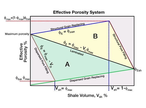
Crossplot of effective porosity versus shale volume, Log analysis of low resistivity and low contrast pays — **Figure 14**: Crossplot of effective porosity versus shale volume

Using the equation for effective porosity as: ϕ_E=V_sh⋅ϕ_Tsh. Juahasz assumes that shale’s bound-water does nor contrubute to effective porrosity, and therefore:

$\phi _{Esh} = \phi _{Tsh} - V_{sh} \cdot \phi _{Tsh} = 0$

Where

ϕ_Esh = Effective porosity in shale

ϕ_Tsh = Total porosity in dhale

V_sh = Shale volume

Crossplot Boundaries and End Points

Juhasz uses the equations that describe different distributions of shale to define key lines on the effective porosity triangles:

Laminated shale only (V_sh=V_L): $\phi _E = \phi _{max} - V_L \cdot \phi _{max} \cdots \cdots$ Triangles A and B
Dispersed shale only (V_sh=V_D): $\phi _E = \phi _{max} - V_D \cdots \cdots$ Triangle A
Structural shale only (V_sh=V_S): $\phi _E = \phi _{max} \cdots \cdots$ Triangle B

Where:

V_L = Shale volume: laminar

V_D = Shale volume: dispersed

V_S = Shale volume: structural

V_sh = Shale volume

ϕE= Effective porosity

ϕ_max= Maximun porosity: clean sand porosity

Triangle A, which is used only to describe laminated or dispersed shales, is defined by three points:

Sand: ϕ_max, such that V_sh=0%
Shale: ϕ_Esh, such that V_sh=100%
Sand: in which all porosity is entirely filled by dispersed shale: (ϕ_Esh⋅ϕ_max), such that V_sh= ϕ_max

Triangle B, which is used only to describe laminated or structural shales, shares two of three points in common with the other triangle:

Sand: ϕ_max, such that V_sh=0%
Shale: ϕ_Esh, such that V_sh=100%
Sand: in which all grains have been entirely replaced by structural shale:
[ϕ_max+(1−ϕ_max)⋅ϕ_Esh], such that V_sh=1 − ϕ_max

Choosing the Appropriate Triangle

The evaluation begins by selecting the appropriate shale distribution triangle.

Similar to the previous discussion on the total porosity system, we use shale volume and effective porosity data pairs to calculate the theoretical value of V_L which should be required to satisfy the effective porosity in the case of laminated shale distribution:

$V_L = \dfrac{\phi _{max} - \phi _E}{\phi _{max}}$

A comparison of the above V_L to the actual shale volume will lead to one of three results:

1. V_sh=V_L, in which only laminated shale is present, such that:

$\small {V_D} = \small {V_S} = 0$

Porosity of the sand laminae is expressed by the equation:

$\phi _{Es} = \phi _{max}$

In this case, all data pairs of ϕ_E and V_sh will plot along the common hypotenuse shared by both triangles.

2. V_sh<V_L, in which only laminated or dispersed shales are present in this case, all data pairs plot within Triangle A, such that:

$V_L = \dfrac{\phi _E - \phi _{max} + V_{sh}}{1 -\phi _{max}}$

The volume of dispersed shale within the sand laminae is expressed as:

$V_{Ds} = \dfrac{V_{sh} - V_L}{1 - V_L}$

Juhasz then expresses the porosity of the shaly sand laminae by the relation:

$\phi _{Es} = \dfrac{\phi _E}{1 - V_L}$

3. V_sh>V_L, in which only laminated or structural shales are present in this case, all data pairs plot within Triangle B, such that:

$V_L = \dfrac{\phi _{max} - \phi _E}{\phi _{max}}$

The amount of structural shale can be determined by relating it to total bulk volume:

$V_S = V_{sh} - V_L$

$V_D = 0$ (No dispersed shale will be plotted within Triangle B)

The shale content of the sand laminae are derived from V_s corrected for the reduced bulk volume of the sand laminae:

$V_{Ss} = \dfrac{V_S}{1 - V_L}$

The porosity of the sand laminae are again expressed by the equation:

$\phi _{Es} = \phi _{max}$ or

$\phi _{Es} = \dfrac{\phi _E}{1 - V_L}$

Hydrocarbon Saturation in the Effective Porosity System

Assuming that all hydrocarbons are contained within the sandstone portion of a shaly sandstone, Juhasz expresses the hydrocarbon saturation in the sandstone as:

$S_{hEs} = \dfrac{\phi _E \cdot S_{hE}}{(1 - V_L) \cdot \phi _{Es}}$

Where:

S_hEs = Effective hydrocarbon saturation in the sand

ϕ_Es= Effective porosity in sand

S_hE = Effective hydrocarbon saturation

V_L = Shale volume: laminated

Guidelines for When to Use the Different Log Interpretation Methods

When the clay is dispersed or when the clay or shale distribution is not known, use either the dispersed clay or Fertl method.
If the shale is laminated, use the Simandoux, dual water or Juhasz method.
When the clay is dispersed and the resistivity of the dispersed clay is known to be the same as the adjacent shale (bioturbated or turbidite shaly sands), use the Simandoux or dual water method.
If the resistivity of the dispersed clay in the shaly sand is known, or you feel comfortable in assuming that the resistivity of the dispersed clay (R_cl) is equal to 0.4 times (Fertl and Hammack, 1971) the resistivity of the adjacent shale (R_sh), then use the Simandoux or dual water method.
In areas where formation water resistivities are high (R_w > 0.1 ohm-m), water saturations calculated by the Fertl (1975) and the dispersed clay methods should be used with caution, because it is assumed in both equations that R_sh > R_w; however, in shaly sands with high formation water resistivities, this assumption may not be true. If R_sh ≅ R_w, use the dual water method.
When cation exchange capacity data is available, use the Waxman-Smits-Thomas method, irrespective of the shale distribution type.